T. Suntola and P. Lievonen

Mathematical Visualizations

by Petri Lievonen

This page is a work in progress.

We are building a research consortium and collaboration around these topics. Physics Foundations Society is a registered association (3066327-8) in Finland. Current research partners include a project in the philosophy of physics at the University of Helsinki and the Cosmological Section of the Czech Astronomical Society, where Suntola is a foreign member.

Contact: [email protected], [email protected]

On this page

• Cosmological Timescales
• Local Timescales and Gravitational Effects
• Energy-Momentum Relations
• System Structures and Inertial Work

Interactive Mathematical Illustrations of Proposed Cosmological Timescales

Historically, zero-energy universe was studied by Arthur Haas, Richard Tolman, Dennis Sciama, Edward Tryon, Pascual Jordan (see Kragh 2015, p. 8, for some context and mathematical formulation), among others (perhaps Dicke, Dirac; see Kragh 2015b). The principle and its specific mathematical form was also mentioned by Richard Feynman in his Lectures on Gravitation, p. 10 – which is based on notes prepared during a course on gravitational physics that he taught at Caltech during the 1962–63 academic year – closing that section with the comment that

All of these speculations [described here] on possible connections between the size of the universe, the number of particles, and gravitation, are not original [by me] but have been made in the past by many other people. These speculators are generally of one of two types, either very serious mathematical players who construct mathematical cosmological models, or rather joking types who point out amusing numerical curiosities with a wishful hope that it might all make sense some day.

The following interactive illustrations are based on a novel interpretation of the zero-energy principle – leading naturally to bouncing cosmologies (see also 1,2,3) and to serious rethinking of the common usage of SI units, especially the second, the metre and the kilogram, along with the various derived units – and its application to physical theory development by Tuomo Suntola as documented in his work The Dynamic Universe (2018).

Assuming that the energies of matter and gravitation are in balance in a finite universe, reminescent of an action principle and analytical mechanics,

$$m{c}_0^2-\frac{GMm}{R}=0,$$

which we refine to a differential equation by defining

$$c_0(t)=\frac{dR}{dt},$$

the following relations hold (see 1,2,3,4,5,6,7,8).

Figure 1. Nonlinear development of the scale of the universe, using effective M = 1.758×10⁵³ kg (corresponding to a current mass density of around 4 or 5 ×10^–27 kg/m³). Under this model, the current 13.8-billion-year-old universe is 13.8 billion light years in radius (hyperradius of a multidimensional space, specifically the 3-sphere). In the hypothetical linear hypertime units (scaled to current years), it corresponds to approximately 9.2 billion hyperyears of positive age.

Figure 2. The theoretical velocity of expansion (hypervelocity) has been enormous in the past, suggesting that also processes have evolved with a great energy and pace. In this model, the hyperspeed of light is linked to the expansion velocity of space, and is currently the defined 299 792 458 m/s (in both standard and hypertime units). See also commentaries about the JWST findings, where, for example, “The objects are spinning super fast” in the early universe.

Note that as $R$ is even in $t$ (see also the matching exponent of $2/3$ in the scale factor in matter-dominated era), it naturally suggests a past symmetric development (bouncing cosmology, see also 1,2,3,4,5,6), but instead of a Big Bounce, more resembling a collapse due to its own gravity “through the eye of the needle” (perhaps related to Planck length scale; see also 1,2,3,4) to “the other side” (where some properties could get inverted, such as giving rise to the matter-antimatter asymmetry). These relations and their potential consequences could also be studied as purely algebraic definitions without physical extrapolation, perhaps represented as a scalar field.

It is interesting that by assuming (or deriving from Maxwell's equations, as Suntola has done) that the Planck constant $h$ has an inner structure where the hypervelocity $c_0$ is a factor,

$$\hslash ={\overline{h}}_0{c}_0=m_P{l}_P{c}_0,$$

one attains an exotic cosmology where the frequencies of physical oscillators, such as clocks (which also define the SI second) follow the development of the scale factor $R$ and its hypertime derivative $c_0$ in just the right fashion for the speed of light to be experienced as constant throughout the evolution of the universe. Also the fine-structure constant, which affects much of the particle physics also in the early universe, is then still a true constant

$$\alpha =\frac{e^2{\mu }_0}{2h_0}\approx \frac{1}{1.1049\cdot 4{\pi }^3},$$

where $e$ is the elementary charge, ${\mu }_0$ is the vacuum magnetic permeability, and $h_0$ is the hypothetical intrinsic Planck constant, assumed as constants.

Figure 3. In this model, the SI second gets longer (in hypothetical hypertime units) during the course of the evolution of the universe. This is dictated by the zero-energy principle. It means that the hyperfrequencies of atomic oscillators, for example, are linked to the development of the cosmos via the fundamental energy conservation laws. Note that possible inhomogeneous developments have not been taken into account here; this is the aggregated model at the largest scales.

Figure 4. For a local observer evolving along with the rest of the universe, the speed of light (with other related processes) is experienced as a constant. This kind of attempt at modeling the observer and the observed together from a hypothetical hypertime perspective is quite unique to the Suntola framework, and offers possibilities for clarifying different timescales across the sciences.

Figure 5. In SI units, we arrive at a R = ct universe due to the constancy of the speed of light. One should be vary of quick comparisons to standard interpretations and cosmology models derived from Friedmann equations (in the context of general relativity), as here the age vs. scale vs. redshift vs. brightness -relations are quite different and derived from conservation of energy and geometrical first principles. The behavior displayed here is linear and scale-free (see also renormalization group), which is conceptually prudent as we should be able to infer the same developmental history even in the far future without living at a preferred moment of time on some S-curve, and the expansion depicted here affects then potentially even the smallest gravitationally bound spatial scales “here-and-now”. In this model, there is no dark energy nor acceleration, and in hypertime units, the expansion is actually decelerating in a very regular fashion, as was evident in Fig. 2 . The model seems to even have some empirical support in supernova observations, provided one uses the redshift-brightness relations derived from this model (see Figs. 8,9,10 later). Note that the redshift-inferred age of far JWST observations would be quite different and perhaps favorable to galaxy development under this model (mentioned briefly also later on this page).

So under this model, it seems that one should be quite careful in distinguishing between different timescales (see also cosmic time and age of the universe), as otherwise one may mix units in a confusing fashion. The second is involved in SI units such as joules [kg$$m${}^2$/s${}^2$] and watts [kg$$m${}^2$/s${}^3$], and in physical constants such as $c$ [m/s] and $G$ [m${}^3$/$$kg$$s${}^2$], which can be viewed as varying or constant, depending on one's conception of the second. Thus Suntola prefers to do the calculations starting from the largest scales (under this model), that is the entire cosmological history (displayed above, see also for geology). On largest scales there is a hypothetical constant timescale, which is called hypertime $t$ here. Note that the gravitational constant $G$ and total mass M [kg] is conserved under this model, and the model prefers to treat scale factor $R$ as a dimension measured in meters [m], as the definition of the meter stays constant and consistent across space and time – cosmologically retarted light travels the same physical distance (for example, 1 m) when measured with cosmologically retarted oscillators, as the SI second is defined as a count of 9 192 631 770 of specific clock cycles, and the SI meter as the distance light travels during the count of those cycles. However, there are important caveats in more local settings, as discussed later.

Devising a simplistic geometrical explanation for the apparent uniformity of the cosmos (see, e.g. horizon problem) leads one to consider finite, positive curvature geometries and hyperspheres, especially the expanding 3-sphere, for contemplation as the global zero-energy structure of the universe. It has many desirable mathematical properties, such as it supporting exactly three linearly independent smooth nowhere-zero vector fields, allowing consistent global rotations and making crosscuts along the great hypercircle arc between any two points in the ordinary three-dimensional space (the volumetric surface of the 3-sphere), still having that extra zeroth hyperdimension along the hyperradius as a degree of theoretical freedom at every point of interest. For more information about these spaces, see my presentation on Clifford algebras and other topics at the Physics & Reality 2024 conference (and 1,2,3,4). Note also how from the viewpoint of general relativity, Sean M. Carroll mentions that in the Robertson-Walker metric on spacetime, for the closed, positive curvature case “the only possible global structure is actually the three-sphere”. Let's also appreciate that the current observed spatial flatness (cosmological curvature parameter) is inferred under the standard cosmology model, but if the model changes, so may also the interpretations of observations regarding the shape of the universe.

So combining, the assumptions lead from having the motion and gravitation in a fascinating eternal balance (Fig. 6 below), to beautiful logarithmic spirals that the radiative tangential momenta of light may trace with us in a four-dimensional hyperspace, see Fig. 7 next. The horizon problem is thus inverted, and while the observable universe can still be conceptualized around us, from a hypothetical hyperspace perspective everything (including us) is really at the “edge” of the multidimensional space, which is developing at tremendous velocity towards future possibilities, while also grounded by everpresent gravity and various consequences of past actions (but note that causality is a difficult subject; classical physics is clearly being preferred here, and contingencies are being investigated). Under this model, when we look out into the distant space (tangentially), we are actually looking in to the center of the hyperspace – and conceptually also past it towards the eternities.

Figure 6. Energies of matter (motion in the hyperspace) and energies of gravitation (integrated throughout the whole of cosmos, where gravity is assumed to act along the tangential surface of the hyperspherical space causing the gradient of the hyperscalar potential to point along the “virtual” hyperradius due to positive curvature of the space) have been quite formidable in the past, but always sum to zero. Note that these are hyperenergies, as in standard units the energies are constant due to the changing SI second.

Figure 7. Assuming that the velocity of light in ordinary tangential space is linked to the radial velocity of space (expanding zero-energy volumetric surface), the resulting logarithmic spirals of light on a circle crosscut view of the hyperspace display manifestly scale-free behavior. With these definitions, the form of the light geodesics are independent of the velocity of light, so these fundamental relations hold in both standard and hypertime units. Predicted redshift z of light from a hypothetical emitter along with other important geometric relations are printed on the interactive diagram. The great distances could even appear discretized here, as conceptually we could see very, very dim traces of revolutions of light around the universe on top of each other, each fulfilling the whole sky due to spherical lensing effects (at redshifts 1 + z = e^nπ, where even and odd n mark antipodal points).

Zooming in to the present in Fig. 7, and making a variation to the hyperradius (and thus to hypertime), could give us a glimpse how light cones and different foliations (slices or leaves) could perhaps be mapped to this presentation, provided one keeps in mind the distinction between position and momentum spaces (see also various astronomical kinematic velocities and their current estimates, where Solar velocity with respect to CMB is notable; see also comoving coordinates and local standard of rest), as in the gravity model studied here, electromagnetic radiation has momentum only in the tangential direction of the 3-sphere (that is, “ordinary three-dimensional space”) and gets a “free ride” along the expansion, having no rest mass in the vacuum. This crucial idea is studied a bit further in relation to the energy-momentum relations at the bottom of this page.

Also discussions on the nature of causality could get interesting, as the picture above presents naturally the energy and information being attainable only as conveyed by the logarithmic spirals at the speed of light (at a maximum), but there are also other geometric relations present – due to the expanding spherical space, spirals have met in the past and will meet also in the very distant future, even if at the present most light cones seem separate. Also the model suggests that there is a theoretical possibility for some scalar potentials being instant across the universe “right now” in some sense, similar as in standard gravity the static field potential is “instant” (the force between inertial charges pointing towards the instant location, not to the retarted location, due to how the Lorentz-transforms operate, also in general relativity, but see [1,2,3,4]). As a force is the gradient of energy, and changing the energy necessitates conveying (abstract) mass (under this model), that can only propagate at the speed of light, these questions about the character of physical potentials, principle of locality, and possible “action at a distance” are complicated and under study. Already that short note about action at a distance contains suggestive ideas, such as John Wheeler and Richard Feynman “interpret Abraham–Lorentz force, the apparent force resisting electron acceleration, as a real force returning from all the other existing charges in the universe”, reminescent of Mach's principle, but for electrodynamics. In the model under study here, it is assumed that as one cannot suddenly move any mass instantly, there is also necessarily always some slowness and inertia with regard to moving (or changing) potentials, irrespective of their range. These important but difficult structural questions are also discussed a bit more nearer to the bottom of this page.

Notice that in that same circle crosscut view of the hyperspherical space, there is the prediction for apparent brightness $L$ (see also apparent magnitude), using the geometrically motivated optical distance $D$ (see the same Fig. 7 above) with inverse distance squared dilution, together with a single $1/(1+z)$ apparent power dilution due to expansion of the space (the energy is conserved in an expanded wavelength of light):

$$\text{Using}D=R\frac{z}{1+z},$$$$L=L_z\frac{D_0^2}{D^2}\frac{1}{(1+z{)}^3}=L_0\frac{D_0^2}{D^2}\frac{1}{1+z}=L_0\frac{D_0^2}{R^2}\frac{1+z}{z^2},$$

the actual form of which is still contested. Note that there is the added complication of greater energetic state of the earlier universe, which affects both absolute luminance $L_z$ and its dilution during the expansion, so actually when calculating in linear hypertime units there is an additional dilution of $1/(1+z{)}^2$, that is exactly canceled by $(1+z{)}^2$ higher luminance in the past, so the formula using only a single $1/(1+z)$ dilution factor in relative units holds when calculating with standard absolute magnitudes.

This very constrained and almost parameterless form fits very accurately to Type Ia supernova observations (Lievonen & Suntola, in preparation, see Fig. 9a), or at least as accurately as luminosity distance in standard cosmology, but there has to be extra $1/(1+z{)}^2$ dilution added to the model to fit with observations. Suntola maintains (Suntola 2018, pp. 264–275) that due to historical reasons, this extra dilution is actually in the processing of supernova observations (specific to conventions in multi-bandpass filter comparisons, see Figs. 9c and 9d later), but not in observed reality, so the following modified formula that fits the observations should be regarded as phenomenological model, but not physical:

$$L=L_z\frac{D_0^2}{D^2}\frac{1}{(1+z{)}^5}=L_0\frac{D_0^2}{D^2}\frac{1}{(1+z{)}^3}=L_0\frac{D_0^2}{R^2}\frac{1}{z^2(1+z)}.$$

The following is a research preview (Lievonen and Suntola, in preparation):

Figure 8 (a,b,c,d). Modeling Type Ia supernova observations (latest released DES 5-year data) by integrating a redshifted supernova spectral flux distribution template (Hsiao et al. 2007) over each filter (g,r,i,z) bandwidth at each redshift z (emitted far in the past), and applying the derived apparent brightness L(z) relation to arrive at physical flux predictions (max envelope curves) through each filter at the current hyperradius R. Calibrated fluxes (in log fluxcal units) through DECam g,r,i,z filters are plotted against redshift z (redshift_final or zHD in the DES-SN5YR release) up to z = 1.2, using color alpha channel to indicate the approximative peakmjd date. Photflag detect, no quality cuts, SNIa candidates filtered to a selection of CIDs. Fluxcal has been inverse transformed in the data release to correspond to top-of-atmosphere fluxes normalizing for galactic extinction, host galaxy surface brightness differences, among other effects. We do not know yet whether some wavelength-dependent processing has been done to the observations in the release – the fluxcals correspond to AB magnitudes with a zero-point of 27.5. Predictions using several different 1/(1 + z)ⁿ dilution factors have been plotted as envelope curves, where the red curve corresponds to the phenomenological brightness model above, whereas the blue curve would be the more correct (geometrically motivated above) brightness model. The model predicts quite nicely the maximum envelope curve of the supernova observations (the peak of each vertical light curve), with essentially just a single parameter R (apart from the values in the empirical spectral template at 10 parsecs, SNIa absolute magnitude of –19.253 from Pantheon+ that is needed as the SED template has been apparently normalized to zero mag in max B-band, and a standard conversion factor of 48.60 applied in transforming the predictions in erg/s/cm²/Å physical units to fluxcal units in AB magnitudes): the current hyperradius R of 13.8 billion light years.

Figure 9a. SNIa distance modulus mu (MU_SH0ES vs. zHD from Pantheon+ data release) supports the model studied here. Hubble–Lemaître diagrams are among the most important tools in modern empirical cosmology. In the model under study, there is only a single parameter, the current hyperradius R = c/H₀ = 13.8 bln ly (in parsecs to be compatible with absolute magnitude distance D₀ = 10 pc). Interestingly, the corresponding H₀ = 70.8 km/s/Mpc would be in the middle of the current Hubble Tension. The standard “–2.5 log” comes from the definition of magnitudes. The lone observation with the blue error bar at z = 2.903 is arXiv:2406.05089. Note that there may be some horizontal and vertical bias due to interactive plotting; this is a research preview.

Figure 9b. According to Suntola analysis, there may be unintentional extra (1 + z)² dimming in all the reported SNIa data across all the surveys globally due to the way how multi-filter observations are combined to a single magnitude value, instead of predicting the observed physical fluxes through each filter separately (see the next two figures). The plot above displays instead the (1 + z)² brightened data (for magnitudes, less is brighter), which fits then nicely to the hypergeometrically motivated brightness prediction, and could thus depict the true bolometric magnitude. This line of inquiry is under investigation. The button on the top right corner resets the plot.

Figure 9c. Suntola maintains (2018, pp. 264–275) that due to historical reasons, there is an unintentional extra (1 + z)² dilution in the processing of supernova observations (specific to K correction conventions in multi-bandpass filter fusion in the standard cosmology, the red curve above), but not in observed (bolometric) reality. This would obviously affect the very basis of dependable observations in all the Hubble–Lemaître diagrams on SNIa worldwide, and would have serious consequences for the empirical basis in astrophysics. See, for example, how the diagram is the very first figure (in log z scale) in the Big-Bang Cosmology chapter in the Review of Particle Physics. SNIa absolute magnitude of –19.253 here is from Pantheon+. The estimated peak magnitudes through different filters (dashed curves) are from Tonry et al. (2003, Table 7), and they seem to each saturate at the proposed true curve (in blue) when redshift matches each filter's optimal wavelength. Filter designations BVRIZJ (here) and griz (in Figs. 8 a–d) correspond to different photometric systems, where the older ones are usually described by energy-based transmission curves, whereas modern systems are count (photon) based. Note that the aforementioned Tonry et al. table is in Vega magnitudes, which have different reference flux densities for each filter band, so the above analysis may also turn out to be misleading or incorrect. There may also be some horizontal and vertical bias due to interactive plotting; this is a research preview.

Figure 9d. Analytical curves (dashed lines) displaying the effect of K correction on a blackbody source observed through idealized filters, resulting in a (1 + z)² dimming envelope curve. Inspect Hogg (2002, p. 4), Hsiao et al. (2007) (along with his thesis), and kcorrect documentation, together with (1,2) for analysis by Suntola. As an example, the black dots are his analysis of the K correction values to B-band at peak from Riess et al. (2004), Tables 2 and 3. However, verifying the chain of analysis here has proven to be difficult, so the black dots here should be taken as only illustrative. But it does not sound impossible to get to the roots of this already quite well defined and studied issue, as the physics of photometric filters is a well-known subject. This would require the expertise of specialists in magnitude systems and their calibration (reported zero points, etc.), and other related subjects (such as chromatic corrections), however, to disentangle the factors. Note also that the differentials of frequencies and wavelengths are related by df = –(c/λ²) dλ, so there are several quadratically varying factors present in redshifted wavelengths (and AB magnitudes are defined on constant flux density per unit frequency, as opposed to unit wavelength, see image). The data analysis pipelines are usually well reported, but there may be important details in the complex procedures applied even to the reported raw data, and may be crucial in the eventual understanding of dilemmas such as Figs. 8 (a–d). We are studying Brout et al. (2019), Sánchez et al. (2024), and their references such as Guy et al. (2007) for this purpose.

All in all, if this total geometric model turns out to be valid and useful in many contexts, it could have interesting consequences for our discussions about time, space, and motion in general. For example, the so-called cosmological time dilation, where supernova light curves are empirically observed as taking a longer duration in the past (dilated by $(1+z)$), would have a simple geometrical explanation: propagating electromagnetic evidence in the form of light from hyperradius interval between the beginning and end times of a supernova gets exaggerated by exactly $(1+z)$ during the expansion, as is evident from the logarithmic spirals above (Fig. 7). For a local observer, the supernova would have occurred in a standard time interval, but in linear hypertime units (where the observer is modeled along with the observed) the process would have gone faster in the past, and slower in recent history, and all this would be seen as lengthening of the light curve by $(1+z)$ compared to the observations nearer to us, exactly as is observed.

Figure 10a. SNIa light curves (vertical lines in Fig. 8c, DECam i filter) plotted from low redshift (blue in the back) to high redshift (red in the front). The vertical axis is the same (log fluxcal), but now the horizontal axis is time (days), aligned on approximative peakmjd reported in the DES 5Y data release. On higher redshifts (red, emitted in the distant past) the light curves are observed as broadened, the supernova explosion seemingly taking a longer duration. We acknowledge this may not yet be the best representation, as usually one fits a computational light curve model to this raw, noisy data, so the relation is then more clear. Also one needs to ascertain that this apparent cosmological time dilation is not an artefact of dimmer observations at higher redshifts; the logarithmic scale should keep the shapes of the curves comparable. In addition, at each redshift, stretch is also related to peak brightness in a different way (see Phillips relationship).

Figure 10b. Shrinking the duration of light curves by 1/(1 + z) seems to homogenize them. This would be in line with the model studied here, where the expansion of space would cause the hyperradius interval between the emitted light at the start and end events of the supernova to get exaggerated by exactly this amount by the time of observation. See the text for some details, and study Fig. 7 closely to familiarize with the proposed geometric relations affecting these phenomena. Note also that with the definitions above (related to hypervelocity of light, and thus the hyperradial velocity affecting the SI second and rapidity of processes in general), the hyperradius interval traveled during the SNIa explosion is constant, irrespective of the time when the explosion happened in the cosmic history.

It seems that it is standard practice to use both the stretch factor (displayed above in Fig. 10a), and the so-called color in regression analysis when producing the distance modulus magnitude data displayed in Fig. 9a (see Scolnic et al. 2022, p. 4, from Pantheon+ papers):

Each light-curve fit determines the parameters color ($c$), stretch ($x_1$), and overall amplitude ($x_0$), with $m_B\equiv -2.5{\log }_{10}(x_0)$, as well as the time of peak brightness ($t_0$) in the rest-frame B-band wavelength range [emphasis added]. To convert the light-curve fit parameters into a distance modulus, we follow the modified Tripp (1998) relation as given by Brout et al. (2019a):

$$\mu =m_B+\alpha x_1-\beta c-M-{\delta }_{\mu \text{-bias}}$$

where $\alpha$ and $\beta$ are correlation coefficients, $M$ is the fiducial absolute magnitude of an SN Ia for our specific standardization algorithm, and ${\delta }_{\mu \text{-bias}}$ is the bias correction derived from simulations needed to account for selection effects and other issues in distance recovery. For the nominal analysis of B22a, the canonical “mass-step correction” ${\delta }_{\mu \text{-host}}$ is included in the bias correction ${\delta }_{\mu \text{-bias}}$ following Brout & Scolnic (2021) and Popovic et al. (2021). The $\alpha$ and $\beta$ used for the nominal fit are 0.148 and 3.112, respectively, and the full set of distance modulus values and uncertainties are presented by B22a.

It could prove out to be problematic that the distance and redshift is used implicitly (via stretch and color) already in the data releases, where the cosmological models are then fitted, instead of predicting the observed spectral energy flux densities directly (as would be preferable in physics). It seems that when comparing different cosmological models (using predicted brightnesses and their inferred distances) using SNIa data, some theoretical assumptions may have been baked in already, as the language mentioning rest-frames also suggests in the above quote. Observe also how Anderson (2022, p. 2) motivates K-correction:

The K−correction accounts for the difference between the (observed) apparent magnitude of a source and the apparent magnitude of the same source in its comoving (emitter) inertial frame. [emphasis added] The difference is caused by two effects: a systematic shift of the spectral energy distribution (SED) incident on the photometric filter (bluer parts of the emitted SED pass through the photometric filter), and a dimming effect due to the fixed-width filter appearing compressed when viewed from the source. [emphasis added]

The luminosity distance itself should take care of all the physical attenuation factors during the expansion, so it would predict the observations. Now it almost seems as if using the co-moving distance in the luminosity distance causes extra $(1+z{)}^2$ dimming for predictions, which is then inadvertently matched by utilizing the K correction in producing the matching $(1+z{)}^2$ dimmer observations. Using light-travel distance (lookback time distance) in luminosity distance (in place of co-moving distance) would then match with non-K-corrected data (as light travel distance is approximately $(1+z)$ longer and would produce approximately $(1+z{)}^2$ power amplification compared to standard luminosity distance).

It would be illuminating if the $(1+z{)}^2$ dimming effect of K correction (in Fig. 9d) could be shown or invalidated with the analysis pipelines and data parameters in Pantheon+ (for example, using this table and its sources). This analysis is in progress, but is complicated by the fact that different physics communities intermix discussing photons (in frequency space) and spectral energy densities (in wavelength space), and have different established conventions in analysing and reporting their results. For example, due to aiming for consistency when developing new photometric systems, practitioners keep referring to needing to convert the observations to the same filter band (such as B-band) to be able to make comparisons. Of course this is necessary when comparing various kinds of observations of same kind of static objects (such as stars) through different filters, but it seems that it has then confused the practitioners to think that different observations of distant dynamic supernovae are somehow also comparisons to rest frame B-band absolute magnitude of SN Ia, which should not be the case. When predicting observed brightness, the absolute magnitude (representing luminosity observed in B-band at 10 parsecs, or is it representing total bolometric flux at that distance?) is not for a comparison, it is simply an emission property of the light source needed as a parameter to be able to predict the observed brightness at a longer distance. Aiming to then convert that measurement (in SI units) back to some hypothetical state seems misguided. The physical flux through the filter is what it is.

Contrary to standard cosmology, employing these novel brightness-redshift-scale-age relations under study on this page here, many observations of the James Webb Space Telescope might make more sense under this model: instead of “too early” galaxies at redshift $z\approx 15$ (about 270 million years cosmic time in standard cosmology, see also), that redshift would correspond to about 860 million years (in standard units, and only 140 million hypothetical hyperyears, where processes would have gone much faster during that time), which is plenty more time for galaxy formation. One can study these by setting the scale at the time of emission in the logarithmic spiral plot above (Fig. 7) to observed redshift $z$, and then inspecting the other synchronized plots, such as the first one, that displays both the hypertime and the hyperradius (in billions of light years), from where the standard time can be inferred from.

Various distance measures utilized in reasoning about the dimensions of the observable universe would get updated; the comoving distance would be related to the length of the hyperradius-normalized circular arc in the logarithmic spiral plots above (Fig. 7), and the so-called proper distances would be then related to the non-normalized, expanding arcs between the points of interest.

Instead of integrating out the light-travel distance, the optical distance $D=Rz/(1+z)$, derived and used above, would be much more simpler to manipulate while also more accurate (under this model). It is quite well known that the integral in the light-travel distance has a special point at ${\mathrm{\Omega }}_{\mathrm{\Lambda }}=0.737125$ (when ${\mathrm{\Omega }}_k={\mathrm{\Omega }}_r=0$), where the integral from zero to infinite redshift is equal to 1, and thus the light-travel distance to the edge of the observable universe equals the Hubble distance $R$. This can be calculated by taking the limit $z\to \mathrm{\infty }$ in the integral, arriving at $d_T(\mathrm{\infty })=d_{H}2\mathrm{atanh}({\sqrt{\mathrm{\Omega }}}_{\mathrm{\Lambda }})/3{\sqrt{\mathrm{\Omega }}}_{\mathrm{\Lambda }}$ (using hyperbolic angle addition formula and taking the argument to the limit). Of course, one does not necessarily need to take the limit to infinite redhift to see that the light travel distance approaches Hubble distance $d_H$ (or $R$) with that ${\mathrm{\Omega }}_{\mathrm{\Lambda }}$ parameter value, as redshift z = 1 000, for example, is already quite far to the early universe. So it is interesting that it seems that some of the parameter values in standard cosmology (such as cosmological constant $\mathrm{\Lambda }$ at ${\mathrm{\Omega }}_{\mathrm{\Lambda }}\approx 0.7$, see also), that are claimed to be empirical findings, are quite close to values that can be derived formally just from the chosen mathematical structure of standard cosmology without referring to observations. See also Fig. 1 in Melia & Shevchuk 2012.

Furthermore, a more precise cosmological angular measure $A$ for a rigid object with diameter $a$ would then turn out to be simply

$$\text{Constant object}A=\frac{a}{D}M=\frac{a}{R}\frac{1+z}{z}M,$$

where $M$ is a possible magnification/lensing factor of hyperspherical space (see Michal Křížek, forthcoming; see also their Cosmological Section (in Czech), Cosmology on Small Scales conferences, and Mathematical Aspects of Paradoxes in Cosmology).

What is highly intriguing (and needs a thorough investigation) is that when interpreting observational data using these geometric angular measures, it seems that many astronomically interesting objects, instead, could turn out to be expanding with the space, as the apparent angular size is then

$$\text{Expanding object}A=\frac{a_D}{D}M=\frac{a}{D(1+z)}M=\frac{a}{Rz}M,$$

due to the (hypothetical) current diameter $a$ having been smaller in the past, by $1+z=R/R_S=a/a_D$ (inspect relations in Fig. 7 and compare the above angular measure to observational data in the figure below).

The following figure displays work-in-progress in interpreting these angular measures.

Figure 0x. Predicting apparent angular sizes of distant objects (at each redshift z, in log-log scale). Most of the components in this figure are under development:

• Blue curves predict observed angular sizes of objects that expand with the space. So under this model, it seems as if galaxies expand with the space, which would be contrary to what is the long-time consensus in astrophysics.
• Red curves predict the angular sizes of constant objects. There are various alternative versions for research purposes. The one with a turnover point is the angular diameter distance in standard cosmology (ΛCDM), which does not seem a good predictor for this particular data.
• The possible 3-sphere lensing effect M = ln(1 + z) / sin(ln(1 + z)), predicting peaking at antipodal points, is under study. Note also that such magnification could affect the inferred velocities of distant phenomena.
• The data (open circles and black dots) is from Nilsson, Valtonen, Kotilainen, and Jaakkola (1993, p. 469, Fig. 5). (See also FINCA)
• Interpreting the angular sizes (observed sizes in calibrated pixels) from JWST are under study (the dim ellipsoid at the bottom). There are various factors which can affect the interpretations. There is material, for example, in [1] and [2].

So in this model, the galaxies and planetary systems could be expanding after all (along with the rest of the space, as so-called kinematic and gravitational factors are conserved in this gravitational model), and so would the stars and planets as gravitationally bound objects to some extent. “Electromagnetically bound” systems (Suntola articulation), such as atoms, would not expand along with the space, but “unstructured matter”, which also light represents due to wavelength equivalence of energy of radiation in this framework, would expand and dilute with the space, dictated by the presented zero-energy principle in the evolving universe. See also the works by Heikki Sipilä, such as Cosmological expansion in the Solar System. Finding out the consequences and implications (using the understanding of Suntola framework) is a difficult task, involving thermodynamics and contemplations about elastic SI units, among other interesting questions.

Interactive Mathematical Illustrations of Proposed Local Timescales and Gravitational Effects

The following displays various important proposals contained in Suntola's work. Visualizations are under development.

$$\text{Assuming}m{c}_0^2=\frac{GMm}{R}\text{and}m{c}_r(x,t)\le m{c}_0(t).$$

Local gravitation, in an idealized setting where there is a mass $M_r$ at a distance $r$, is modeled as bending of space to angle ${\varphi }_r$ (in the hyperplane spanned by hyperradius $R$ and a vector along $r$) to maintain the zero-energy balance:

$$c_{0}m{c}_r=\frac{GMm}{R}-\frac{G{M}_{r}m}{r}=\frac{GMm}{R}(1-\frac{M_r/M}{r/R})=\frac{GMm}{R}(1-\frac{G{M}_r}{r{c}_0^2})=\frac{GMm}{R_r}=c_0(m{c}_0\cos {\varphi }_r).$$

So the binding (decreasing) effect of local gravitational energy $-G{M}_{r}m/r$ on the rest energies $m{c}_0^2$ is equivalent to multiplying the rest energies with a gravitational factor $(1-\frac{G{M}_r}{r{c}_0^2})$, that is only slightly less than unity in weak gravity (when $r\gg G{M}_r/c_0^2$) and approaches zero in strong gravitational fields, observed as gravitational time dilation. The effect of the gravitational factor can then be conceptualized as lengthening of the “virtual” hyperradius $R$ to $R_r$ (where the conceptual mass equivalence of the rest of space is following along), specific to that point in space, or equivalently as rotating the hypersurface locally to angle ${\varphi }_r$ with respect to the flat space, the projection of which then contains the necessary effect on rest energy. The rotation is in the hyperplane, so the radial distance differentials along the hypersurface lengthen, whereas transverse components (such as the circumference $2\pi r$ at a radius $r$) stay unchanged. In the process, the venerated $E=m{c}^2$ has been split into hypervelocity $c_0$ (in the unchanged hyperradial direction) and a novel concept of “rest momentum” $m{c}_r$, that represents the locally available rest energy (when multiplied by $c_0$ to convert from momenta to energies, $E=c_{0}m{c}_r$). The reduction cannot be observed locally, due to all the reference energies (and thus SI units) varying in the same proportion in the vicinity.

The tangent of the hypersurface crosscut is then

$$\tan {\varphi }_r=\tan {\cos }^{-1}(1-\frac{G{M}_r}{r{c}_0^2})=\frac{\sin {\varphi }_r}{\cos {\varphi }_r}=\frac{\sqrt{1-{(1-\frac{G{M}_r}{r{c}_0^2})}^2}}{1-\frac{G{M}_r}{r{c}_0^2}},$$

which can be integrated to arrive at the hypersurface crosscut shape of

$$\int \tan {\cos }^{-1}(1-\frac{G{M}_r}{r{c}_0^2})dr=\frac{2G{M}_r}{c_0^2}(\sqrt{\frac{2r{c}_0^2}{G{M}_r}-1}-{\tanh }^{-1}\sqrt{\frac{2r{c}_0^2}{G{M}_r}-1})+C,$$

or integrating from a reference distance $r_0$,

$$\mathrm{\Delta }R={\int }_{r_0}^r\tan {\cos }^{-1}(1-\frac{G{M}_r}{r{c}_0^2})dr=\frac{2G{M}_r}{c_0^2}(\sqrt{\frac{2r{c}_0^2}{G{M}_r}-1}-\sqrt{\frac{2r_0{c}_0^2}{G{M}_r}-1}-{\tanh }^{-1}\frac{\sqrt{\frac{2r{c}_0^2}{G{M}_r}-1}-\sqrt{\frac{2r_0{c}_0^2}{G{M}_r}-1}}{1-\sqrt{\frac{2r{c}_0^2}{G{M}_r}-1}\sqrt{\frac{2r_0{c}_0^2}{G{M}_r}-1}}).$$

Let's also note that in general relativity, the Schwarzschild solution differs from the above by a square root and a factor of two in the critical radius, so integrating GR solution to model the “bending of spacetime in extra hyperdimension” so that the local projection $c_0\cos {\phi }_r$ would correspond to gravitational time dilation $c_r=c_0\sqrt{1-2GM/c_0^2}$ could be achieved instead by surface integral

$$\int \tan {\cos }^{-1}\sqrt{1-\frac{2G{M}_r}{r{c}_0^2}}dr=2\frac{2G{M}_r}{c_0^2}\sqrt{r-\frac{2G{M}_r}{c_0^2}}+C.$$

The following illustrates the resulting hypothesized “dent” $\mathrm{\Delta }R$ in zero-energy surface volume in this idealized setting around a black hole (or any mass center when radially far in weak gravity), measured in meters and scaled to the unit critical radius $G{M}_r/c_0^2$. In an Euclidean four-dimensional space, the direction of virtual hyperradius is always present as orthogonal to any regular space direction, so the diagram should be read as a hyperplane crosscut spanned by the direction of the hyperradius $R$ and a vector along $r$ towards the mass center (in flat space). It is a symmetric picture from which ever direction in ordinary three-dimensional space we approach the mass center. Going forward, this is quite crucial to get consistently operated on, and it has not been formulated in a more expressive language, such as differential geometry or geometric algebra yet. For comparison, the GR solution (where $\mathrm{\Delta }R=c_0\mathrm{\Delta }t$ and $c_r=c_0\cos {\phi }_r$, interpreted crudely under this model) is plotted with a gray dashed line (and dotted line is its artificial extension, as the solution would otherwise end abruptly at the Schwarzschild critical radius, where the projection vanishes, so transforming to alternative coordinates would be needed for comparison there).

Figure 11. The hypothetical dent in hyperspace of the volumetric zero-energy surface (in hyperplane crosscut view) around a mass center M_r according to the ΔR(r) relation above. For a test mass m, the always present hypermomentum (in yellow) along the direction of expansion (hyperradius) is decomposed to two orthogonal components: the momentum of free-fall (equivalent to the escape momentum, in blue), and the local rest momentum (in darker yellow, indicating the local gravitational energetic state and thus the local speed of light in this gravitational model, where the gravitational time dilation and radial stretching of space have been taken into account). Zooming in to the test mass, the even darker yellow represents the local rest momentum when the mass is in actual free-fall from a great distance (thus invariant in its non-inertial coordinate system, see also geodesics), where the motion causes even more time dilation, as if the test mass would be “lifted” slightly from the hypersurface due to speed (see the last equation on this page). In a circular orbit, the kinematic effect would not be as strong, as the orbital velocities are quite moderate. The diagram also depicts with dual vectors on the “underside” of the surface how the virtual mass equivalence of the rest of space could be conceptualized as moving further away as the test mass approaches the mass center; that virtual hyperradial distance R_r has been scaled down from approximative Hubble distance (currently 13.8 billion light years) for visualization purposes. See the text for more details.

The plots below display various velocities related to this gravity model. They are ordered from more global timescale to more local. Specifically, the uppermost plot (Fig. 12a) displays velocities with respect to the flat space (static observer at rest far from the critical radius, but ignoring light propagation delays). From that perspective, which is actually the most common one when we are almost always modeling physical phenomena from far away, the speed of light (middle yellow line) slowing down near mass centers is not too exotic, as that is also the prediction in general relativity. Note, however, that various forms of the equivalence principle are not taken as axioms here, and will most probably not hold in these strong gravitational fields in this gravitational model. The middle diagram (Fig. 12b) relates then the velocities to that local time standard (proper speed of light, that middle yellow line), which changes with gravitational state (distance $r$) and is not affected by the velocities of relatively small masses moving in space. The bottom one (Fig. 12c) relates the velocities to a local free-falling (non-inertial) observer (darkest yellow line), where the additional observer-specific dilation due to motion causes the velocities to be observed as even greater. One may be able to salvage the locally (in “local spacetime patch”) observed invariant speed of light by assuming (or deriving under this model, as will be done later), that actually objects expand uniformly at velocity, thus completely nullifying the effect of extra time dilation at velocity. It does not affect any longer distances (just their appearance), but that locally one will be perhaps able to measure the speed of light as invariant and isotropic (at least for a roundtrip time-of-flight calculation and optical interference studies, which could be affected by this hypothetical expansion at velocity, and also Doppler effects could become relevant). In Suntola studies, first-principles motivations, plausible physical mechanisms, and an understandable worldview are sought after, resulting in quite straightforward mathematics.

Figure 12a. Various velocities at a distance r from a mass center M_r with respect to the flat space. Solid lines display the predictions from the model studied here, whereas dashed lines are their Schwarzschild equivalents (but partly interpreted under this model). The darkest yellow lines are not actually velocities, but plotted here for convenience (it is the combined effect of gravitation and motion in free-fall, resembling the equivalence principle). Yellow lines are related to gravitational time dilation and thus speed of light (in coordinate time). Blue lines are velocities of free fall from a state of rest at a distance, and their radial and hyperradial components are plotted with gray. Red lines are orbital velocities (with no hyperradial component). See text for details.

Figure 12b. The same velocities with respect to the local gravitational state “hovering” at each distance. Many velocities seem to reach the local speed of light, which is extraordinary behavior (and test masses cannot maintain their integrity way before that), so it seems that orbital velocities (in solid red) could be the most characteristic and stable features here. There could be a way to take the orbital velocity as fundamental (so that total diffused mass M_r is really there, in the slow orbits), analyzing some kind of spiraling capture dynamics in the evolving universe. That kind of investigation has not been attempted yet.

Figure 12c. Again the same velocities, but now plotted as observed locally by a free-falling (starting from far away or at orbit) observer at each distance r, taking into account extra kinematic time dilation. This picture is complicated by the fact that locally SI meter seems to expand with velocity (under this model), so actually the velocities are inferred as constant irrespective of own velocity, so the same as in upper Fig. 12b. The same invariance applies when normalizing for observers in circular orbits (calculating the kinematic factor (1 – v²/c²)^1/2 from red orbital velocities in Fig. 12a). This seems to imply that locally matter expands on the move (thus enabling invariant experiments), but also inferred further distances seem to shrink at velocity, as light travels a longer distance in the same locally observed time frame. These figures and their implications are under study.

In blue, there is the velocity of free fall (equivalent to escape velocity), which is related to the sine of the angle of rotation of the hypersurface volume. The velocity of free fall saturates at the speed of light at the critical radius, which seems very nice and regular. However, do note how the “4D-well” (black line in the earlier Fig. 11) extends arbitrarily far in the direction of the hyperradius, possibly even to the origin of the hyperspace where different black holes could be connected (at least in the early history of the cosmos). But as the hyperspherical space is expanding and the hypersurface volume is thus developing vertically in the crosscut picture at the speed of light (by definition of the hypervelocity), it seems likely that a falling object can at maximum stay at the same absolute hyperradius distance, not travel “backwards in time” to the origin. Also the horizontal and vertical components (gray lines) of the escape velocity have been plotted for convenience. The interpretations of the Schwarzschild coordinates (dashed lines, and accompanied velocities) should be treated with caution here, as only some of them are exactly known from GR studies, and in different coordinates (such as using null geodesics), the meaning of critical radius would change considerably. Some Schwarzschild velocities, such as free-fall coordinate velocity (dr/dt) and orbital velocities (red dashed lines, in their “distant observer” coordinate form, “hovering” observer proper form, and an orbiting observer proper form), should be exact according to our knowledge, but even they may contain errors, because we have conflicting information from text books (see also 1,2,3,4). It is of interest that in Schwarzschild coordinates, the Newtonian orbital velocity depicts also the orbital velocity in coordinate time (for a far-away observer), but cannot support stable circular orbits nearer the critical radius (as depicted by the abrupt ending of red dashed line at the photon sphere).

Some special points of Schwarzschild geodesics have been highlighted in Fig. 11, such as between 1.5 (so-called photon sphere) and 3 times the Schwarzschild radius $2G{M}_r/c_0^2$, which are already challenging for sustaining stable orbits in Schwarzschild metric (discussed also briefly later).

In the gravity model studied here, orbital velocities (red line, in circular orbits) stay nice and regular down to the critical radius (Suntola 2018, pp. 142–163). Maximum orbital velocity is attained at four times the critical radius (Fig. 12a). Relative to gravitational state at a distance $r$ (middle plot, Fig. 12b), the maximum orbital velocity is attained at two times the critical radius, which also happens to be the radius for the minimum period for circular orbits, as the calculated period (from the perspective of a far-away observer) is

$$P_r=\frac{2\pi }{c_0}\frac{G{M}_r}{c_0^2}{\left(\frac{G{M}_r}{r{c}_0^2}(1-\frac{G{M}_r}{r{c}_0^2})\right)}^{-3/2},$$

which can be compared to Kepler's third law of planetary motion. In the limit, as $r\to \mathrm{\infty }$, the prediction for the relations between orbital period and orbital radius are equal, as they should. In fact, the familiar relation $P_r^2\propto r^{\prime 3}$ holds with $r^{\prime }=r/(1-G{M}_r/r{c}_0^2)=r/\cos {\varphi }_r$ which is the tangential distance in Fig. 11.

For a local free-falling (non-inertial) observer, the situation is complicated as the velocities seem to increase without limit (as reference frequencies decrease towards zero, affecting SI second), but at the same time the SI meter expands (both definitionally and physically, in this model), thus the observational velocities being inferred as constant, and further distances being measured as shrunk as the light travels a longer distance in the observationally same time frame. Also for an observer in a circular orbit (red line in the above figures), the situation is quite remarkable in lower orbits, as the reference frequencies and oscillators come to a standstill the closer one orbits the critical radius, so distances are inferred as warped and shunk in a complicated but perhaps manageable way, but note that the actual orbital velocities seem to come to a standstill, so the kinematic term is approaching unity (no kinematic time dilation). Matter seems to dissolve into some exotic form of mass-energy. Suntola claims that these kind of slow orbits (see the same red line from a point of view in the distant flat space in Fig. 12a, and compare to the spatial picture in Fig. 11) maintain the mass of the black hole – it is quite a different picture than a pointlike singularity, as here photons can climb very slowly also up from the critical radius (which is half of that of the Schwarzschild event horizon).

Some claims, such as the escape velocity having a well-behaving form down to critical radius, could simplify the common physical picture in the long term. However, the velocities plotted to local time standards imply some rather exotic physics, where the velocity of free fall can meet and exceed the local proper velocity of light (which is decreasing near mass centers in this gravitational model), as Suntola claims that in a free-fall, the relativistic mass increase is not necessary, as the energy is taken from the hyperrotation of the space itself (maintaining the zero-energy principle). It could mean that on the atomic level, new kinds of mass-energy conversions could be possible around black holes around critical radius, that are perhaps hitherto undertheorized. Distance $(2+\sqrt{2})G{M}_r/c^2$ is geometrically special in Suntola framework, as there the space has been bended and rotated to exactly 45 degrees with respect to the expanding hyperradius, and it happens to correspond to approximative radius of neutron stars (about 5–11 km, using current estimated variability of neutron star mass).

It is also interesting to plot the surface integral outside of its domain of applicability using complex values, where mathematically the surface seems to have imaginary values (orange line) starting from $-\pi$ inside the critical radius. But note that the spatial and energetic relations as defined have broken down, so care should be taken to make progress in interpreting this.

Figure 13. Plot of the hypersurface integral in the complex domain. One could also compare the figure to the logarithmic integral function and Ramanujan–Soldner constant, but here the association is quite distant. (An even more distant association is in relation to the fine-structure constant, see 1,2,3,4,5, where in the last one the minimum kinematic factor in circular orbit has been experimented with.)

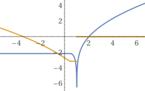
As a mathematical curiosity, also the period formula shown previously can be plotted in complex domain, where the period is pure imaginary inside the critical radius.

When operating far from the critical radius ($r_0\gg G{M}_r/c_0^2$ and $r\gg G{M}_r/c_0^2$), the above asymptotically approaches

$$\mathrm{\Delta }R={\int }_{r_0}^r\tan {\cos }^{-1}(1-\frac{G{M}_r}{r{c}_0^2})dr\approx \frac{2G{M}_r}{c_0^2}(\sqrt{\frac{2r{c}_0^2}{G{M}_r}}-\sqrt{\frac{2r_0{c}_0^2}{G{M}_r}})=2\sqrt{\frac{2G{M}_r}{c_0^2}}(\sqrt{r}-\sqrt{r_0}),$$

which can be used to approximate the volumetric surface shape (the hyperradial dimension) in many calculations. For example, Suntola utilizes semi-latus rectum ℓ as a reference distance $r_0=a_0(1-e_0^2)$, where $a_0$ and $e_0$ are (projections of) orbital elements in flat space, to calculate characteristic hyperradial deviations, such as between apsides, where $r_{min}=a_0(1-e_0)$ and $r_{max}=a_0(1+e_0)$ (see semi-major and semi-minor axes), to arrive at the approximative hyperradial distance range of

$$\mathrm{\Delta }R=2\sqrt{\frac{2G{M}_r}{c_0^2}{a}_0}(\sqrt{1+e_0}-\sqrt{1-e_0})$$

during an (approximative) Keplerian orbit.

It is interesting how the resulting prediction for the rate of period decrease of two bodies orbiting one another (thus emitting gravitational radiation) seems more compact in this gravity model than in general relativity, even though they are both employing approximations. The DU solution is (Suntola 2018, pp. 162–163)

$$-⟨\frac{d{P}_b}{dt}⟩=\frac{54\sqrt{2}\pi G^{5/3}{m}_1{m}_2(m_1+m_2{)}^{-1/3}}{c^5{(1-e_0^2)}^2}(\sqrt{1+e_0}-\sqrt{1-e_0}){\left(\frac{P_b}{2\pi }\right)}^{-5/3},$$

whereas GR presents

$$-⟨\frac{d{P}_b}{dt}⟩=\frac{192\pi G^{5/3}{m}_1{m}_2(m_1+m_2{)}^{-1/3}}{5c^5{(1-e^2)}^{7/2}}(1+\frac{73}{24}{e}^2+\frac{37}{96}{e}^4){\left(\frac{P_b}{2\pi }\right)}^{-5/3},$$

which are perhaps surprisingly similar (which is reassuring, as they are derived using quite different means). However, they have very different predictions when orbital eccentricity $e\to 0$ (circular orbit), as DU predicts invariant periods for circular orbits, whereas GR predicts (at least for the above approximation) that also circular orbits decay and emit gravitational waves. The actual modeling machinery behind these claims (what kind of physical binary situations do the models apply to, and what is the effect of approximations made) and their observational evidence are under investigation, to prevent too early conclusions.

I recommend taking a moment here contemplating the gravity of the above statements.

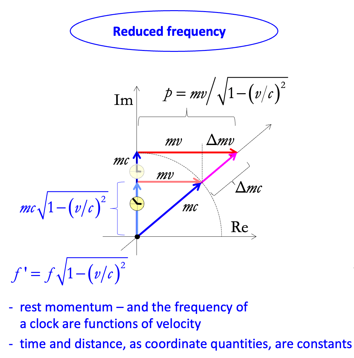
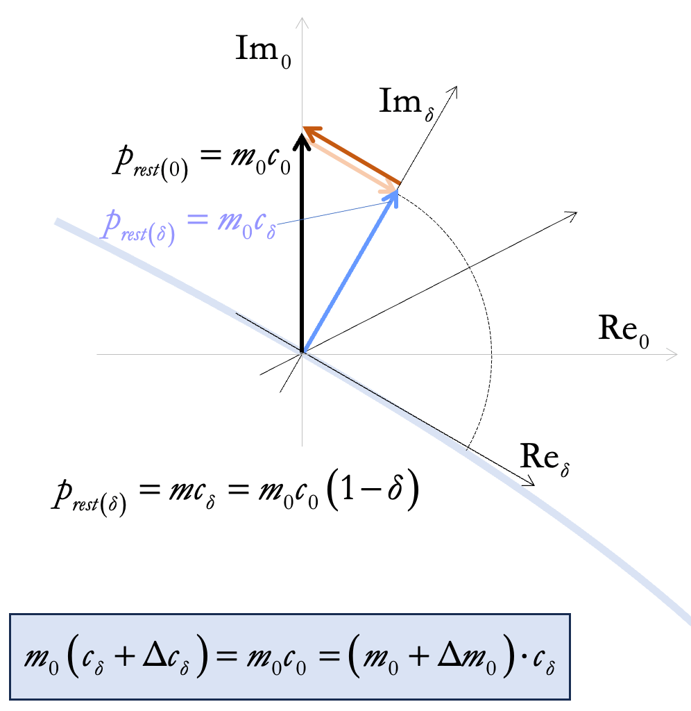
With this construction, the “rest momentum” $m{c}_0$ is decomposed in free fall into two orthogonal components: $m{c}_r$ is the local reduced rest momentum in the bended space at a distance $r$, and $m{v}_{esc}$ is the momentum of abstract free fall, or alternatively the escape momentum, that would be needed to escape back to flat space (see the components in Fig. 11):

$$(m{c}_0{)}^2=(m{c}_r{)}^2+(m{v}_{esc}{)}^2={\left(m{c}_0(1-\frac{G{M}_r}{r{c}_0^2})\right)}^2+(m{v}_{esc}{)}^2.$$

Solving the above for $v_{esc}$ using $G{M}_r/r$ at the Earth surface, results in the correct escape velocity of 11 180 m/s. In such a calculation it is not completely clear, however, why the applied $c_0$ is the current defined $c$ (299 792 458 m/s). It is a bit difficult, but seemingly achievable, to analyze the situation across several time scales. It seems that at least on weak gravity, one can “correct” the locally defined $c$ with a factor greater than one, and then carry out the calculation above, arriving at the escape velocity in terms of that “corrected” timescale, which can then be converted back to escape velocity in the local timescale (where $c$ is as defined) by dividing the factor away – resulting in the same as above.

When taking the gradient of the scalar potential – again in an idealized setting around a single large mass, as is usual when analysing orbital dynamics (sums of these potentials has not been analyzed apart from discretizing the space to nested energy frames) – it seems that local gravitational force gets augmented with a cosine factor due to distance $r$ being defined in a flat (unbended) space, whereas resulting forces display the locally apparent tangential distance in the bended space, and can be projected back to flat space:

$$F_r=\frac{G{M}_{r}m}{{(r/\cos {\varphi }_r)}^2}\cos {\varphi }_r=\frac{G{M}_{r}m}{r^2}{(\cos {\varphi }_r)}^3=\frac{G{M}_{r}m}{r^2}{(1-\frac{G{M}_r}{r{c}_0^2})}^3.$$

In addition to distance $r$ and tangential distance $r/\cos {\varphi }_r$, there is also the distance along the volumetric surface towards some mass center. Their meaning and usage is not yet completely clear, but Suntola (2018, pp. 207–216) has made considerable progress in interpreting various empirical effects, such as Shapiro time delay (with respect to Mariner 6 and 7 experiments), in this framework. For example, usually radial light travel time (in coordinate time) can be simply calculated by integrating (see also and compare also to Eddington–Finkelstein coordinates)

$$\frac{1}{c_r}\int \frac{1}{\sqrt{1-\frac{2G{M}_r}{r{c}_0^2}}}dr=\frac{1}{c_0}\int \frac{1}{1-\frac{2G{M}_r}{r{c}_0^2}}dr=\frac{1}{c_0}(r+\frac{2GM}{c_0^2}\ln (r-\frac{2GM}{c_0^2}))+C.$$

Here, instead, the form of signal propagation duration between radial coordinates can be calculated using (see also)

$$\frac{1}{c_r}\int \frac{1}{1-\frac{G{M}_r}{r{c}_0^2}}dr=\frac{1}{c_0}\int \frac{1}{{(1-\frac{G{M}_r}{r{c}_0^2})}^2}dr=\frac{1}{c_0}(r+\frac{GM}{c_0^2}(2\ln (r-\frac{GM}{c_0^2})-{(\frac{r{c}_0^2}{G{M}_r}-1)}^{-1}))+C,$$

which gives very similar predictions when far from critical radius (and can be truncated to simpler algebraic forms).

It is also quite straightforward to derive predictions for orbital periods using this kind of geometric reasoning, as Suntola has done, and that was also briefly displayed above.

We are also studying the implications of the above to relativistic mechanics, where it is well-known that Newton's second law is modified to

$$F=\frac{d}{dt}\frac{mv}{\sqrt{1-\frac{v^2}{c^2}}}=\frac{m}{{(1-\frac{v^2}{c^2})}^{3/2}}a,$$

whereas in the model studied here, it seems that it is further modified with the effect of local gravity ($c_0/c$) and movement of “parent” frames ($m$ is reduced, as studied later on this page), that can usually be ignored in local physics. Then the more accurate law would be

$$F=\frac{c_0}{c}\frac{m}{{(1-\frac{v^2}{c^2})}^{3/2}}a,$$

which could have implications for the equivalence principle, but needs further study to disambiguate the scalar, 1D, 2D, 3D, and 4D components, and analyze the possibly varying measurements units involved.

These discussions on hypothetical reduced rest momentum and local timescales (variable proper speed of light, as observed from the distance), lead us to kinematic and gravitational time dilation, that are both routinely taken into account in satellite operations. To see the components, study, for example, these two images (from popular sources [1,2], with texts and markings kept verbatim, and the model studied here plotted on the image):

Figure 14a. From the source image: “Satellite clocks are slowed by their orbital speed, but accelerated by their distance out of Earth's gravitational well.” The model studied here reproduces rather well the standard picture in relativity. The image (with its terminology and plotting) is reproduced here in verbatim, but DU predictions have been plotted over it as is, matching the graph very precisely without any alterations. Green line is calculated as a simple fraction of the clock frequencies (r₀ is Earth radius, see also middle yellow line in Fig. 12a). Red line is also a simple fraction (orbital velocity v_r is calculated using an accurate formula, see red line in Fig. 12a, and v₀ is the velocity at the equator). The total effect on hyperfrequencies of clocks (blue line) is just a simple fraction of the product of the aforementioned effects – thus Suntola proposes that gravity is actually multiplicatively separable (!), where the “rest momentum” mc₀ is modulated by both the gravitational factor and the kinematic factor. Green dotted line is a crude estimation of gravitational time dilation inside Earth with linearly increasing density and only each inner shell affecting the potential energy (as usual when integrating a scalar potential in 3D).

Figure 14b. From the source image: “Daily time dilation over circular orbit height split into its components. On this chart, only Gravity Probe A was launched specifically to test general relativity. The other spacecraft on this chart (except for the ISS, whose range of points is marked "theory") carry atomic clocks whose proper operation depend on the validity of general relativity.” (The emphases in the original.) The simple equations are exactly the same as in the previous figure, just the scales of the axes are different, so the figure evidently gives support to both GR and DU, and they seem certainly valid and useful models in these domains of applicability (observed parameter ranges). Compare to the more complicated equations usually presented, where the factors do not have as straightforward interpretations as this model seems to have here. Note also how in the proposed factorized structure of gravity, possible common factors from “larger frames” will cancel away when taking the fractions. The dashed gray line is a total time dilation prediction for a purely vertical displacement over the equator, where the velocity is calculated to match ground velocity for static hovering. It then meets the total orbital time dilation for geostationary orbits, as it should. See also other interactive illustrations of time dilation in space.

Note that the experimentally confirmed slight gravity speedup (gravitational time dilation) of clocks seems to imply that the speed of light is necessarily also slightly higher up there, as the “speed of light in a locale is always equal to $c$ according to the observer who is there” (see gravitational time dilation). The same source continues, that according to general relativity, “[t]here is no violation of the constancy of the speed of light here, as any observer observing the speed of photons in their region will find the speed of those photons to be $c$, while the speed at which we observe light travel finite distances in [different gravitational states] will differ from $c$.” Interpreting these effects properly is also important for understanding gravitational redshift, for example (studied a bit later here). The effects are ordinarily quite small, so in many cases (such as GPS), the propagation delays are calculated with a constant velocity of light (contrary to what general relativity seems to recommend above), and it seems that the various dynamic corrections routinely applied (such as for the atmospheric delays) are enough to result in very accurate calculations. There is also the added complication of extinction lengths being just a few millimeters in atmospheric (i.e. non-vacuum) densities (which, however, is just a miniscule effect considering how far the signals get to travel in space, but it affects reception).

The above pictures are present even in the Lunar distance calculations. Often data analysis summaries mention exotic considerations such as Lorentz contraction of the Earth and the Moon, but fail to emphasize that Shapiro time delay is routinely added to computations (see Battat et al. 2009, p. 34), which enables calculating with a hypothetical constant speed of light:

The range model used to analyze the data presented here [for millimeter-precision measurements of the Earth-Moon range] was built upon the publicly available JPL DE421 Solar System ephemerides, from which the positions and velocities of the centers of mass of the Earth and Moon (among other Solar System bodies) can be interpolated. In addition, the range model estimates the position of the ranging station with respect to the center of mass of the Earth and the retro-reflector array position with respect to the center of mass of the Moon. The relativistic Shapiro time delay of light is included [emphasis added], as is the refractive delay through the Earth’s atmosphere, as prescribed by Marini & Murray (1973), though annual averages of the meteorological data, rather than their instantaneous values, are used. The range model, however, is incomplete and can produce drifts in the O−C residuals [...]

So it seems that in actuality, many pictures where light is depicted as propagating with a constant velocity in space (see, for example, 1, 2), are misrepresenting the reality − what is actually observed, and how it is also theorized in general relativity, imply that speed of light slows down slightly near large masses, and radial distances are stretched due to curvature of space. Unfortunately the Shapiro time delay or its meaning for speed of light measurements is not discussed at all in the most definitive SI standards documentation, such as the Mise en Pratique for the definition of the metre in the SI (search for “lunar” and “Moon”), prepared by the Consultative Committee for Length (CCL) of the International Committee for Weights and Measures (CIPM). It is as if the incorrectness of calculating with a constant speed of light is not realized even by most experts. Our current diagnosis is that the necessary procedures routinely applied in scientific instrumentation and technologies of measurement, have been abstracted with terms such as "Shapiro time delay" or "relativistic corrections", which obfuscates their important physical implications for the phenomena under study. The effects of gravitation are small, but they seem to exactly then match with observed gravitational redshift also near Earth surface (but there are dual accounts with respect to changing propagation velocity or changing frequency, depending on the perspective used).

Note also that the orbital speed slowdown (kinematic time dilation in Figs. 14a,b) is not calculated with respect to each observer, but with respect to the Earth-centered inertial (ECI) coordinate frame (see, for example, geocentric celestial reference system (GCRS) and Geocentric Coordinate Time TCG). All the system components are eventually referred to a common coordinate time scale. So judging from this picture, it seems quite evident that the reciprocity of time dilation is not true in most physical settings (outside of thought experiments in special relativity, or in experiments where the temporal and spatial scales are so small that these effects can be ignored in some otherwise symmetric setting as if the space was empty). According to these pictures, if a clock is taken to a higher satellite orbit where it has less orbital velocity, its hyperfrequency will be sped up (interpreting the kinematic factor), and if a clock is lowered to a lower satellite orbit where it needs to have more orbital velocity to stay on orbit, its hyperfrequency will be slowed down (again interpreting just the kinematic factor). This happens from the point of view of this common frame irrespective of any observers, and there cannot be reciprocity of kinematic time dilation here, as observed from these satellites (or anywhere else, for that matter), the situation cannot somehow reverse without major paradoxes appearing down the line. With a slowed down clock, one necessarily measures the other velocities as higher, not the other way around as would be needed for reciprocity. We are happy to discuss any empirical evidence proving otherwise, but for now, we do not have reasons to believe that warping or contracting the space, rotating coordinate systems, or some other hypothetical effect would somehow salvage the reciprocity here. So for now, these are treated as common confusions due to apparently mixing event-centric kinematic and properly system-centric dynamic (i.e. energy conserving) descriptions, and will be studied later on this page.

When a signal is transmitted to or received from space, also Sagnac effect is important. When discussing GPS, McCarthy and Seidelmann (2018, p. 273) tell simply that

The third effect [in addition to the gravitational and kinematic effects] is the Sagnac delay, which is caused by the motion of the receiver on the surface of the Earth due to the Earth’s rotation during the time when the signal is on its way from the satellite. This delay is computed in the GPS receiver [...] [and] can be as large as 133 ns.

There are many ways the treatment of Sagnac delay is motivated in the literature, but Suntola has calculated that treating it simply as the lengthening of the propagation path during the transmission of the signal due to the receiver moving along with the rotating Earth, results in the most straightforward mathematics and its physical interpretation.

So it is quite evident that those Figs. 14a and 14b certainly warrant studying and discussion. What is the role of the approximations and structural explanations here (Lievonen & Suntola B, also in preparation). The images are in weak gravity (where the gravitational factor is near unity), and also still quite far from relativistic velocities (thus the kinematic factors are also near unity), but the components of time dilation are already empirically visible. In mathematical terms, it is then interesting that calculating the total time dilation (in blue) using a sum of time dilations (the conventional way),

$$\frac{f-f_0}{f_0}=(\frac{f^{\prime }\sqrt{1-\frac{2G{M}_r}{r{c}_0^2}}}{f^{\prime }\sqrt{1-\frac{2G{M}_r}{r_0{c}_0^2}}}-1)+(\frac{f^{″}\sqrt{1-\frac{v_r^2}{c_0^2}}}{f^{″}\sqrt{1-\frac{v_0^2}{c_0^2}}}-1),$$

and using a factorized structure instead (the model studied here),

$$\frac{f-f_0}{f_0}=\frac{f^{\prime }(1-\frac{G{M}_r}{r{c}_0^2})\sqrt{1-\frac{v_r^2}{c_0^2}}}{f^{\prime }(1-\frac{G{M}_r}{r_0{c}_0^2})\sqrt{1-\frac{v_0^2}{c_0^2}}}-1,$$

really result in practically equivalent predictions, but very different interpretations of experiments, different theory structures, and different extrapolations to strong gravitational fields and associated high kinetic energies.

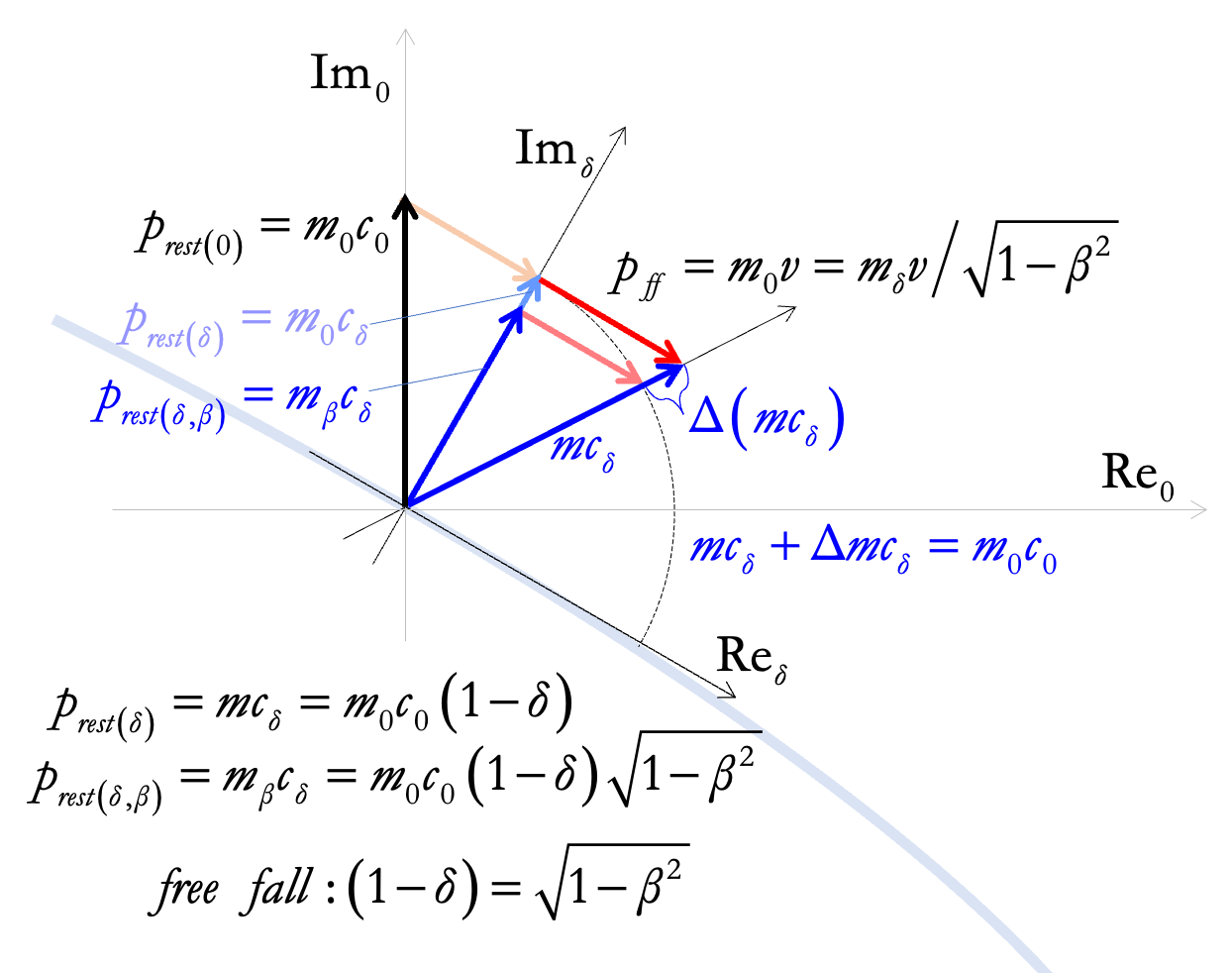
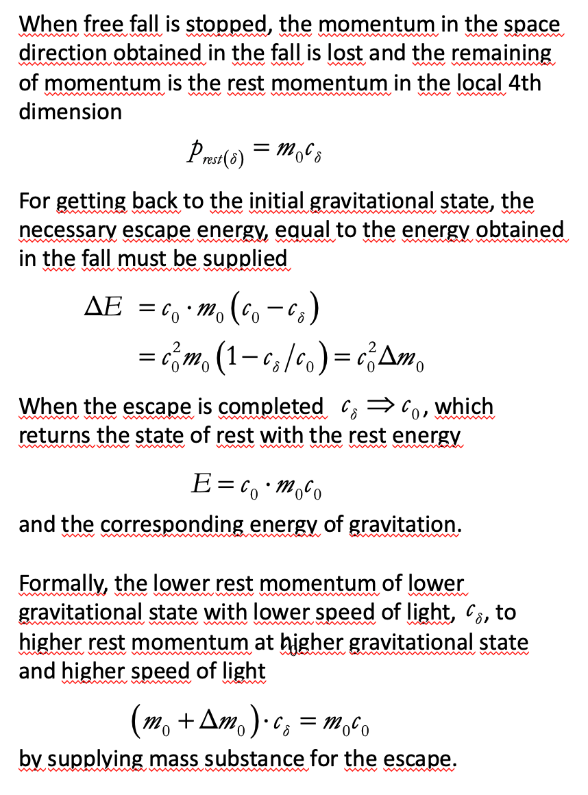
As a brief of things to come in terms of the hypothetical gravitational model studied here, the hyperfrequencies of clocks and oscillators are predicted to follow the reduction in local “rest momentum”, due to both motion and gravitation effects in the local “energy frame” (see again Fig. 14a), which is regarded as an objective and totality-oriented, as opposed to observer-oriented, concept.

The reduction is modeled as two factors (kinematic and gravitational), formally affecting the “rest mass” and “speed of light” separately, but actually modulating the “rest momentum” as a total:

$$f(p,r)\propto {\overline{m}}_v{c}_r=m{c}_0\sqrt{1-\frac{v^2}{c_r^2}}(1-\frac{G{M}_r}{r{c}_0^2})=m{c}_0\sqrt{1-\frac{v^2}{c_r^2}}-m{c}_0\sqrt{1-\frac{v^2}{c_r^2}}\frac{G{M}_r}{r{c}_0^2}.$$

Note the striking similarity (when multiplied by $c_0$ to get from rest momentum to rest energy) to the mathematical forms in relativistic Lagrangian mechanics, where the form of the Lagrangian is

$$L=-m_0{c}^2\sqrt{1-\frac{{\dot{\mathbf{r}}}^2}{c^2}}-V(\mathbf{r},\dot{\mathbf{r}},t).$$

It is related to kinetic energy, potential energy, and total energy, and it makes the relativistic action functional proportional to the proper time of the path in spacetime.

Note that the critical radius $r_D$, evident in the above formula for frequencies and in previous Figs. 11–12a,b,c, is half of that as in Schwarzschild radius $r_S$. It does not have much of an effect in normal gravity situations (DU and GR predictions are essentially equivalent, note also that the scale of the images of black holes should be contrasted with the critical radius which is smaller), but it could turn out to have interesting consequences nearer the critical radius, as Suntola has analyzed. Compare also how Schwarzschild metric has a potential for much more regular structure in DU, as in Schwarzschild coordinates (where in radial great circle crosscut $\varphi =d\varphi =0$),

$$\frac{d{s}^2}{c^2}=d{\tau }^2=(1-\frac{2G{M}_r}{r{c}^2})d{t}^2-{(1-\frac{2G{M}_r}{r{c}^2})}^{-1}\frac{d{r}^2}{c^2}-\frac{r^{2}d{\theta }^2}{c^2},$$

whereas in DU space, the above could be interpreted as

$$\begin{array}{rl}\frac{d{s}^2}{c^2}=d{\tau }^2& ={\sqrt{1-\frac{2G{M}_r}{r{c}^2}}}^{2}d{t}^2-{\sqrt{1-\frac{2G{M}_r}{r{c}^2}}}^{-2}\frac{d{r}^2}{c^2}-\frac{r^{2}d{\theta }^2}{c^2}\\ & \approx {\left((1-\frac{G{M}_r}{r{c}_0^2})dt\right)}^2-{\left({(1-\frac{G{M}_r}{r{c}_0^2})}^{-1}\frac{dr}{c_r}\right)}^2-{\left(\frac{rd\theta }{c_r}\right)}^2,\end{array}$$

which has a nice quadratically symmetric aesthetic to it. It could be related to the so-called harmonic and isotropic coordinates that Steven Weinberg utilized in his impressive work on Gravitation and Cosmology (1972), but this connection has not been studied properly yet. In the above comparison, the direction of the approximation (which one is more accurate on theoretical and empirical grounds) is contested (see Suntola 2018, p. 158). In DU, the $(1-G{M}_r/r{c}_0^2)$ form is exact (when $r\ll R$ and $M_r\ll M$, as otherwise $r=\theta R$ and higher-order terms, such as for $e^{-1/\theta }$ or $1/(1+1/\theta )$, may become important, where $\theta$ is in terms of global 3-sphere in Fig. 7, not in terms of these local 2-sphere coordinates), derived already early on in this section.

The following diagram illustrates how close the approximations are to each other, especially when far from critical radius.

Figure 15. The critical radius in the gravitational model of Suntola (the endpoint of solid green line) is half of that as the well-known Schwarzschild radius (the endpoint of the green dashed line). Note that the Schwarzschild solution is an exact solution to the Einstein field equations in general relativity describing the gravitational field outside a spherical mass, and it cannot be altered arbitrarily, so Suntola proposes that there are fundamental differences between these models. The green lines above agree to very high precision when far from the critical radius, as is usually the case. For example, the critical radius of the Earth is a few millimeters, so the Earth surface is multiple orders of magnitude further away in the above plot. See Fig. 14a,b, where the same colors have been used for the same factors (green is gravitational factor, red is orbital velocity factor, and blue is their product). As a bonus, light red is the inverse of the kinematic factor in a circular orbit, and therefore depicts the expansion of Bohr radius (and thus solid matter in general) due to increasing Compton wavelengths when gaining velocity, under this model. Note that in SI units, local length measurements are constant due to the expanding SI meter, as studied later on this page. How all this would affect complicated effects, such as frame-dragging (see 1,2), has not been analyzed.

In the Schwarzschild metric, it is well-known that one can study the time and space coordinates separately in idealized situations. For example, by setting spatial differentials to zero ($dr=d\theta =d\varphi =0$), the above results in

$$d\tau =\sqrt{1-\frac{2G{M}_r}{r{c}^2}}dt,$$

which in DU proposition is

$$d{\tau }_r=(1-\frac{G{M}_r}{r{c}_0^2})dt.$$

It depicts the gravitational time dilation at a distance $r$, so for example 1 second in coordinate time ($dt$), is less in proper time $d\tau$ at a distance of $r$ from the mass center, as the gravitational factor is less than one (and approaches zero towards the critical radius). In terms of SI units, it is then definitionally true that the frequencies of Cesium atomic clocks must decrease accordingly (in coordinate time, that can be taken as hypertime here), as the second is defined as a count of 9 192 631 770 of such cycles of radiation. So instead of modeling time intervals, it seems more real to attempt to model the frequencies and their accompanying physics as such, so the units of measurement stay valid. Otherwise we risk mixing different duration seconds together, as "$dt$" and "$d\tau$" have different units, even though they both seem to use SI seconds – they are defined properly only locally, and the same goes for constants that use the SI units, such as $c$ here. So actually, it could be illuminating to treat the relation between $d\tau$ and $dt$ as applying between physical hyperfrequencies instead:

$$f_r=(1-\frac{G{M}_r}{r{c}_0^2})f_0=f_0\cos {\varphi }_r,$$

where ${\varphi }_r$ is not the Schwarzschild coordinate, but a local angle to extra spacelike hyperdimension, as described earlier on this page. The factor must apply equally to all frequencies (the spectrum) for the physics to stay valid, as gravitational time dilation is universal (it affects all phenomena in physics). Consequently, the local speed of light $c_r$ (in hypertime) must decrease accordingly, so the SI system works (as for a meter, the wavelength $\lambda =c_r/f_r$). The above is modeled as the local speed of light affecting the rest energies (which stay constant in local SI units, but change in hypertime units), which in turn affects the characteristic oscillations as is observed in Fig. 14b, for example.

Also for the spatial coordinates the same treatment (setting now $dt=0$) reveals something relevant about the structure of the Schwarzschild solution (but ignoring the important signs here, this is just the spacelike spacetime interval):

$$ds=cd\tau ={\sqrt{1-\frac{2G{M}_r}{r{c}^2}}}^{-1}dr+rd\theta ,$$

which in DU proposition is

$$ds=c_{r}d{\tau }_r={(1-\frac{G{M}_r}{r{c}_0^2})}^{-1}dr+rd\theta .$$

Here we could have divided the metric with local $c_r$ for clarity (as then the metric measures time intervals of light propagation in different directions), and it displays how radial distance differentials are affected by the radial coordinate. Distance [m] divided by velocity [m/s] is duration [s]. Other directions than the radial stay classical (distances on an ordinary sphere). For radial distance, it is then simply

$$ds={(1-\frac{G{M}_r}{r{c}_0^2})}^{-1}dr=\frac{dr}{\cos {\varphi }_r},$$

showing how the radial distances stretch along the hypothetical hypersurface, when the model is embedded in the extra spatial hyperdimension.

Both of these effects – gravitational time dilation, and radial stretching of space – were depicted before in Figs. 11 and 12. Let's acknowledge that this is very unorthodox treatment of the metric here, and as the actual tensors have not been decomposed here with matrix square roots, it is also very non-rigorous. Also treating spacetime intervals as compared to the coordinate time in the distance (as opposed to between different relative observers), may not point out all the difficulties here, but also in standard treatments the $dt$ time intervals are then related to the gravitational state of the observer at $r_0$ simply by dividing by $\sqrt{1-2G{M}_r/r_0{c}_0^2}$, which means division by $(1-G{M}_r/r_0{c}_0^2)$ here, exactly as was done in Fig. 14a,b.

Also usually the radial light propagation is calculated by using null geodesics (setting proper time $d\tau$ to zero),

$$0=\sqrt{1-\frac{2G{M}_r}{r{c}^2}}dt-{\sqrt{1-\frac{2G{M}_r}{r{c}^2}}}^{-1}\frac{dr}{c},$$

which results in (see also)

$$\frac{dr}{dt}=(1-\frac{2G{M}_r}{r{c}^2})c,$$

but it is then the same as simply projecting the light propagating along the hypersurface at velocity $\sqrt{1-\frac{2G{M}_r}{r{c}^2}}{c}_0$ to the radial direction by taking its cosine component $\sqrt{1-\frac{2G{M}_r}{r{c}^2}}\left(\sqrt{1-\frac{2G{M}_r}{r{c}^2}}{c}_0\right)=dr/dt$. In DU terms, it is then $(1-\frac{G{M}_r}{r{c}_0^2})\left((1-\frac{G{M}_r}{r{c}_0^2})c_0\right)$, so

$$\frac{dr}{dt}={(1-\frac{G{M}_r}{r{c}_0^2})}^2{c}_0.$$

Thus this decomposition here seems to result in comparable analysis to relativistic effects, as the light geodesics seem to follow the hypersurface with empirically correct time delays, for example. Thus we feel that in spite of this quite evident incompleteness here compared to the body of knowledge accumulated during the decades on research on general relativity (such as differential geometry and spacetime basis transforms), there may be something really relevant about physical relativity here, as also scalar projections are often indicative of the systems under study (compare to eigenvalues and eigenvectors, and the symmetric and inner products are prevalent even between multidimensional spaces). Thus the research program here is continuing.

One could take a look at the local and delayed velocities in Schwarzschild geodesics, keeping in mind that in DU space,

• $\sqrt{1-r_S/r}\approx (1-r_D/r)$, as the critical radius $r_D$ is half of $r_S$,
• $1/\gamma \approx \sqrt{1-v^2/c_r^2}$, where the usage of local velocity $c_r$ is not completely clear (and when nesting energy frames, it gets more complicated as the $c_0^2$ in gravitational factor $(1-G{M}_r/r{c}_0^2)$ is more accurately $c_0{c}_r^{\prime }$, where the usage of $c_r^{\prime }$ is even more complicated),
• momentum is decomposed into orthogonal components in hyperspace which can be locally hyperrotated, so often projected with $\cos {\varphi }_r=(1-r_D/r)$ or its inverse $1/\cos {\varphi }_r=1/(1-r_D/r)$ (in contrast to the radial component and scalar time), while the space itself is expanding in the hyperradial direction at the hypervelocity $c_0$,
• signals propagate at local proper speed $c_r$ along the volumetric surface dictated by the zero-energy condition, thus being affected by both the decreased velocity by $(1-r_D/r)$ and greater radial distance due to the curvature (which results in the empirically correct Shapiro time delay), while the emitters and receivers are in different energetic states which also affect observations, and
• in abstract free-fall starting from far away, motion and gravitational factors become equal (reminescent of the equivalence principle, where “gravitational time dilation $T$ in a gravitational well is equal to the velocity time dilation for a speed that is needed to escape that gravitational well”, but not exactly the same), $\sqrt{1-v^2/c_r^2}=(1-r_D/r)$, thus allowing simply squaring the gravitational factor to get the factor ${\sqrt{1-r_S/r}}^2=(1-r_S/r)\approx (1-r_D/r{)}^2$, relating the predictions to local time standards, as was done in some of the velocity plots above. This detail could be the key in interpreting the differences between the standard gravitational models, such as GR, and the model studied here, as here the free-fall is only gravitationally present at each distance $r$, not always kinematically. Relativity allows defining any reference frame, and here we are most often not looking from the point of view of a local, freely falling reference frame, which is treated more like a special situation here. Inspect these early images to get a glimpse of the ideas under study: a, b, c, d, e.

This list above is by no means exhaustive, but displays the difficulties ahead due to accidental complexity, which results almost by definition from applying apparently simple ideas (in isolation) to complex problems. Iterating and recursing on partially overlapping concepts and definitions may hinder seeing the essence in the ideas, which in the case of DU almost always stem from the zero-energy principle in a spherically closed space. Also, the scope of conceptual problems with respect to comparing the formulas, is under study, as the underlying postulates about the nature of time, space, and motion are obviously quite different in different propositions, which each naturally aim to be internally coherent and valid without compromising on empirical correspondence and relevance. As an example, the equivalence principle is most often formulated in terms of derivatives (forces), where the boundary conditions are then lost (or they are forbidden, see discussion on absolute space and time), whereas Suntola thinks that energies (and thus integrals, where forces are then derivatives or gradients) are fundamental, and then boundary conditions are essential (however large or miniscule, such as global curvature, they may be, but they are there and may be necessary for making theoretical progress).

The alleged rather complicated nesting of the common energy frames proposed by Suntola (2018, p. 125 for example) and consistency of the procedure in terms of both spatial and temporal effects is not yet clear. There is considerable interest in understading various experimental setups and their theoretical interpretation (see 1,2,3), as carried out under the umbrella of modern searches for Lorentz violation, or studying the physics of Michelson-Morley resonators, for example. See also the classical internet resource on the experimental basis of Special Relativity from The Original Usenet Physics FAQ, hosted by John Baez.

Do note that even though “In small enough regions of spacetime where gravitational variances are negligible, physical laws are Lorentz invariant in the same manner as special relativity” (see Lorentz group), the thought-experiment regions where the gravitational potential is constant are shrinking rapidly due to empirical results enabled by recent advancements in technologies of time measurement. Optical clocks resolving centimeters in height are technically ready for field applications, such as monitoring spatiotemporal changes in geopotentials caused by active volcanoes or crustal deformations, and for defining the geode (see, for example Takamoto, M., Ushijima, I., Ohmae, N. et al. 2020).

As for the physicality and reality of relativistic effects – see Pulsar Timing Arrays, for example, which seem to empirically imply that

[T]he fact that the Earth is moving on an elliptical orbit around the Sun, and hence at varying distances [and at varying orbital velocity], means that every clock on Earth experiences a varying gravitational potential [and thus varying energetic state] throughout the year. This leads to seasonal changes in clock rates that affect all clocks on Earth simultaneously. Astronomy can, hence, provide an “independent” time standard that is unaffected by effects on Earth or in the solar system. The key in providing such an astronomical time standard are objects called “pulsars”. Pulsars are compact, highly-magnetized rotating neutron stars which act as “cosmic lighthouses” as they rotate, enabling a number of applications as precision tools. (Becker, Kramer and Sesana 2018)

In Suntola studies, these effects are considered as physically here and there at this very moment, meaning that one would need to really ponder on the meaning of the SI second (and accompanying metre, kilogram, and other fundamental units) with respect to these observations. Consider also Fig. 14b, where satellites are orbiting Earth, but the same effects are present when Earth is orbiting Sun, and we are making experiments from the point of view of the "satellite Earth" with globally dilated time. As the speed of light is empirically measured as constant and isotropic, but using evidently varying clocks, it would imply that the proper speed of light at a distance changes from the inertial frame of reference point of view. Suntola has studied the idea that going further into larger and larger spatial and temporal scales, there is a specific kind of cosmological timescale, where these local timescales could be derived from.

There may be a possibility to model SR length contractions as theory-internal constructs necessary for being able to calculate in locally invariant units, but it would also make some claims of SR, such as symmetricity (reciprocity) of time dilation, suspect on these new empirical grounds. Also some established interpretation of measurements, such as the distance between the Moon and Earth being constant during the year, would actually seem to imply that the distance increases when the Earth is closer to the Sun, as otherwise it would not be observed as invariant, when taking into account the effect on clocks of varying gravitational potential and additional orbital velocity affecting the energetic state here on Earth. These serious propositions are under investigation.

Suntola reasons, that as clocks and processes evidently go faster in weaker gravitational field (from the point of view of the barycenter of solar system, where the Pulsar calculations are done), it would imply that the effects should be considered physical. He then proceeds to predict that all matter expands uniformly at velocity (in the respective energy frames with respect to their center-of-momentum frames), so the observations are physically understandable. One way to understand this is by looking at the algebraic chain of relations from the Compton wavelength ${\lambda }_e$ of the electron to the frequency of an quartz oscillator, which is driving the electronics of every atomic clock (see Time: From Earth Rotation to Atomic Physics), and thus needs to be in sync with the observed frequency drop at velocity:

$$f\propto \frac{1}{\lambda }\propto \frac{1}{D}\propto \frac{1}{a_0}\propto \frac{1}{{\lambda }_e}\propto \sqrt{1-\frac{v^2}{c_r^2}},$$

where $D$ is some characteristic length of a quartz crystal used in the clock, the expansion of which (by Lorentz factor) among with all the other matter on the move, would explain the kinematic effect observed as decreased frequency of a moving clock. In experiments, taking the Doppler effects on the emitter and the absorber into account is essential, and seem to match with observations (Suntola 2018). $a_0$ is the Bohr radius, which is often taken as representative of the length scale in condensed matter in general. Whether classical electron radius would be somehow involved, is an open question, as that would need intepreting the scattering experiments done in particle accelerators – the expansion would be rather large close to $c$, as can be seen from the numerical values of the Lorentz factor.

In addition to the kinematic effect, the effect of varying gravitational potential is modeled in Suntola model as affecting the energy of matter too, where algebraically speed of sound in condensed matter is directly proportional to local $c$ (and thus is the frequency of a quartz oscillator, too), as Trachenko (2021, eq. 47) has calculated the upper bound for such velocity of pressure propagation in material:

$$v_u=\alpha \sqrt{\frac{m_e}{2m_p}}c\approx 36100\text{m/s}.$$

Do note that Trachenko explicitly tells that velocity of sound (pressure) in condensed matter does not depend on $c$. It is defined as constant, but the algebraic dependency on $c$ is quite clear, potentially giving a mechanistic explanation (albeit very hypothetical at this point!) for the observed frequency drop of a quartz oscillator in the gravitational potential (see, again, Fig. 14b).

See also the formula for the frequency of a Cesium atomic clock in Uzan (2003), Eq. 81,

$${\nu }_{Cs}=\frac{32c{R}_{\mathrm{\infty }}{Z}_s^3{\alpha }_{\mathrm{EM}}^2}{3n^3}{g}_I\mu \approx 9.2\text{GHz},$$

which is directly proportional to $c$, if the other factors, such as Rydberg constant $R_{\mathrm{\infty }}$, do not depend on $c$ (as it is with Suntola proposition). Expressing vacuum permittivity ${\epsilon }_0$ using vacuum magnetic permeability ${\mu }_0$, and creatively assuming (or deriving from Maxwell's equations using a constraint of emission/absorption during a single cycle, as Suntola has done) that Planck constant $h$ has speed of light $c_0$ as a factor, one attains

$$R_{\mathrm{\infty }}=\frac{m_e{e}^4}{8{\epsilon }_0^2{h}^{3}c}=\frac{m_e{e}^4{\mu }_0^2{c}_0^2{c}_r^2}{8h^{3}c}=\frac{m_e{e}^4{\mu }_0^2{c}_0^2{c}_r^2}{8h_0^3{c}_0^{3}c}=\frac{m_e{e}^4{\mu }_0^2}{8h_0^3},$$

which needs studying with respect to $c$ vs. $c_r$ vs. $c_0$, as usually $c$ is defined as constant and the distinction is not made. See also that the $R_{\mathrm{\infty }}$ above, and thus also the frequency $f$ and ${\nu }_{Cs}$, is directly proportional to electron rest mass $m_e$, and that is allowed to vary (decrease) along with all other masses in moving energy frames in the Suntola framework, as presented below. The constant $h_0$ (units in kilogram meters) is also a novel proposition, which is discussed next.

Interactive Mathematical Illustrations of Proposed Local Energy-Momentum Relations

Matter is modeled as having wave properties, where usage of reduced masses or gravitational effects is not yet always clear, possibly due to historically evolutionary development of the models. There is a promise to unify Compton wavelength and de Broglie wavelength interpretations under a single mass concept, using “intrinsic Planck constant” $h_0$, from where $c_0$ has been removed. See also the presentation by Tarja Kallio-Tamminen. Thus, any mass $m=E/c_0{c}_r$ is considered to have a concise wavelength equivalent form

$${\lambda }_m=\frac{h}{m{c}_0}=\frac{h_0}{m},$$

and any momenta, correspondingly, a wavelength equivalence

$${\lambda }_p=\frac{h}{p}=\frac{h_0{c}_0}{mv/\sqrt{1-v^2/c_0^2}}=\frac{h_0}{m{\gamma }_0{\beta }_0}\approx \frac{h_0}{m{\gamma }_r{\beta }_r},$$

where $c_0$ has been used, but using local $c_r$, as in the last form, should be more correct. Obviously, as usually there has not been much discussion about the effects of gravity on de Broglie wavelength, the last form should be equally fine at this point of theory development. Perhaps the specific wavelength equivalences above could be considered as reduced representations (mean approximations) of some kind of wave number distributions or spectrums in wavelength domain, where the calculated wavelength equivalence is characteristic to that mass. See also the clever treatment of blackbody radiation in the appendix, where wavelength ${\lambda }_T=h_0/k_{0}T$ and frequency $f_T=c_r/{\lambda }_T$ equivalences of temperature $T$ are defined using an “intrinsic Boltzmann constant” $k_0=k/c_0{c}_r$, which could be a powerful idea in the future, especially when interpreting observations related to thermal radiation in the expanding space (see also 1).

Suntola uses the geometric properties of an enormous expanding hypersphere in four-dimensional space to suggest that the reason that a small hydrogen atom can emit 21 cm wavelength light may have its physical basis in this hyperradial expansion at the speed of light, where the wave equivalence of mass and energy may gain new physical meaning, as any point source could trace a path like an elongaged isotropic monopole or dipole antenna in 4D (orthogonal to all 3D spatial directions) due to this sustained “hidden” movement even at rest. Also the geometries of Dirac matrices, which represent 4+1 dimensional Clifford algebras (isomorphic to 2+3 and 0+5 dimensional algebras), could suggest the same. Interactions (emissions and absorptions) would be wavelength-selective (and frequency-selective), not energy-selective, as can perhaps be motivated by using the definitions above:

$$E=hf(=h\frac{1}{\mathrm{\Delta }t})=h_0{c}_{0}f=h_0{c}_0\frac{c_r}{{\lambda }_m}=c_0{m}_{\lambda }{c}_r\approx m{c}^2.$$

This idea would be of great importance when utilizing relations (such as studying wave equations or simply using $f=c/\lambda$) that could change across time and space. At the same time, locally one cannot really discern a difference between a longer wave that is propagating faster, and shorter wave that is propagating slower, so there are interesting possibilities for surprising invariances when dealing with matter waves – also Doppler effects (1,2,3,4) for moving matter (for both sources and receivers) could become relevant, which is an highly intriguing idea.

Doppler formula for observed frequencies in the Suntola framework (see Suntola 2018, pp. 183–193) is

$$f_B=f_{A_0}\frac{(1-\frac{G{M}_r}{r_A{c}_0{c}_A^{\prime }})\sqrt{1-\frac{v_A^2}{c_A^2}}(1-\frac{v_B\cdot {\hat{r}}_{AB}}{c_B^{″}})}{(1-\frac{G{M}_r}{r_B{c}_0{c}_B^{\prime }})\sqrt{1-\frac{v_B^2}{c_B^2}}(1-\frac{v_A\cdot {\hat{r}}_{AB}}{c_A^{″}})},$$

where the gravitational effect (redshift or blueshift), transversal effect (kinematic time dilation), and classical Doppler effect for both sources $A$ and receivers $B$ are combined to a single formula. The formula is easiest to read inspecting one factor at a time, for example the various effects on the source $A_0$, where it is also instructive to think in terms of shortened or lengthened wavelengths (${\lambda }_A=c_A/f_A$). For the receiver, the corresponding effects cause the references to change, so they affect observations inversely (the reference wavelengths are increased at receiver velocity, so absorptions are seen with decreased wavelengths). There are intentionally various velocities of light visible in the formula, which need to be interpreted according to contextual usage, and propagation across nested energy frames brings even more complications, but the insight of Suntola here with regards to light propagation is that from the perspective of hypothetical linear hypertime, the hyperfrequency of light cannot change during the propagation as the exact same amount of oscillations need to be received as was sent (at least for a long duration ideal test light, i.e. from a coherent monochromatic laser as modeled by Maxwell's equations).

In the thinking of Suntola, photons (and the related Planck relation) are related to interactions (i.e. emissions and absorptions), not so much to propagation in vacuum, which changes interpretations of various observations considerably (but note that quantum mechanical descriptions of beam splitters, photon statistics, and many other crucial phenomena have not been analyzed here). For example, then the emitted wavelength is independent of the gravitational state of the emitter (as frequency and speed of light are linked), and the observed gravitational blueshift, where the wavelength is observed as decreased deeper in the Earth gravitational well, is simply due to the speed of light being decreased accordingly (that is also communicated by gravitational time dilation as the speed of light is invariant for a local observer), and thus the oscillations clumping closer together, observed locally as increased frequency even though energy has not been gained. It is a drastically different picture than the usual conception of photons gaining energy when propagating deeper in a gravitational field, even though the local observations are otherwise identical. Note that the reasoning may be more complicated with respect to light emitted in the cosmological past, as there both $c_r$ and $c_0$ have been greater, and in the model studied here, atoms have conserved their dimensions, which is an important constraint in interpreting the emitted and observed wavelengths and the cosmological redshift.

The following illustrations are under construction, displaying the partial equivalence of conventional four-vector (see four-momentum) formalisms with this 4-dimensional Euclidean momentum space utilized here (at least in the hyperplane crosscut of the momentum space), especially the relativistic energy-momentum relation, the mapping facilitated by the Gudermannian function:

$$E_r=|c_0{p}_4|=c_0\sqrt{p^2+(m{c}_r{)}^2}$$$$\tanh w={\beta }_r=\frac{mv}{m{c}_r}=\sin x$$$$\cosh w={\gamma }_r=\frac{1}{\sqrt{1-\frac{(mv{)}^2}{(m{c}_r{)}^2}}}=\sec x$$

Figure 16a. Fundamental energy-momentum relation in the 2D crosscut of the 4D Euclidean space. Note that the proposed reduced rest momentum (vertical hyperradial dimension in the diagram) related to inversion in a 3-sphere is currently unknown to physics, but could give a mechanistic explanation to the kinematic time dilation (Fig. 14a,b) and associated effects. See also the related identities near the end of this page.

Figure 16b. Euclidean and hyperbolic representations of energy-momentum relations plotted to the same diagram. Note that for simplicity in plotting, only unit hyperbola is plotted, and only on one hyperbolic quadrant.

Figure 16c. A stereographic projection (Gudermannian function) relates the different representations in a deep way (via Möbius transformations, i.e. rotations of the Riemann sphere). The integrals display hyperbolic secant, which is exactly the reduced rest momentum above (and sec x is exactly the Lorentz factor gamma). The s is a kind of holographic projection (especially when complex numbers are employed) related to parabolic geometries (n is a nilpotent) and formalisms for wave functions and spin in quantum mechanics (see works of G. Sobczyk for more details here).

Figure 16d. Common hyperbolic picture displays important invariance to hyperbolic basis rotations, the applicability of which across larger spatial scales is contested in Suntola studies. See also the various visualizations from the kinematic (time and distance, see also accelerating observers) perspective, as opposed to these dynamic (energy and momentum) relations. Commonly used abstractions, such as proper velocities, may gain new interpretations by studying these diagrams.

The above interactive figures display hyperbolic (standard in relativity, see also Dirac matter), parabolic (related to nilpotents, dual numbers and thus automatic differentiation), and Euclidean (quite common-sense local view on the volumetric surface of an expanding three-sphere) intepretations of concepts such as the total (relativistic) energy (in red), kinetic energy (red outside the unit circle), relativistic mass increase (in tangential direction due to supplied mass-energy), rest energy (in center-of-momentum frame), “reduced rest momentum” (hypothesized hyperradial effect of motion), “inertial work” (hyperradial component of kinetic energy against the rest of space), etc. I recommend studying the two formulas near the bottom of the page for some insight to the idea of nested energy frames from an internal and external point of view.

Velocity addition formulas (of rapidities or hyperbolic angles) are hypothesized to get augmented by addition of space-like momenta, with energy bookkeeping for time measurement in each nested energy frame. The following figures visualize the effect of a transparent moving (and non-magnetic) medium on light (see Fizeau experiment) in Suntola framework, with adjustable refractive index (vertical dot in the diagram). There are two horizontal black lines: one is the velocity $v<c$ of the moving medium, the other is the velocity $u^{\prime }<c$ of light in medium (when stationary), dependent on the refractive index $n=\sqrt{{\epsilon }_r}>1$ as $u^{\prime }=c/n$. The longest horizontal line (red) is the resultant velocity $u<c$ of light in the moving medium.

Figure 17a. A moving medium with a non-zero refractive index causes its spatial momentum to be added to the momentum of light, in such a fashion that the observed velocity of light in the medium does not exceed the speed of light in vacuum. See the text for some details. Analyzing these kind of situations is important, as they are surprisingly common – generally extinction lengths are very short (only a few millimeters in air, and just a few light years in interstellar space), which affects interpretations of observations and experiments. See also the Abraham-Minkowski controversy.

Figure 17b. In hyperbolic picture it is assumed that any reference frame can be taken as definitive (hyperbolically rotated to its center-of-momentum frame), and while it is conceptually straightforward to just add the hyperbolic angles, it may hinder the dynamic (i.e. the conservation of energy) understanding of the phenomena, encouraging reduction to kinematic, event-centric descriptions. Note that different energies are not plotted properly here yet.

It is quite amazing how close predictions the relativistic velocity-addition formula and this momentum-space construction above give (when $v>0$), see a 3D-plot. However, negative velocities ($v<0$) of a moving medium has not been studied here yet (the two diagrams above may allow it, but they are not robust), nor orthogonal (or other than parallel) movement, which is a clear deficit. Also the hyperbolic picture should be modified to display energies correctly, as now it is just a kinematic picture using unit hyperbola (as velocity-addition formula applies to hyperbolic angles). See Suntola (2018, pp. 218–221).

Photons (electromagnetic radiation) do not carry rest momentum (in vacuum), so their momenta is pure spacelike (horizontal in the Euclidean picture, isotropic lightlike in hyperbolic picture), and they get “free ride” along the hyperspace expansion without carrying complex momentum – compare to aforementioned logarithmic spirals (Fig. 7) further up on this page.

One may also keep in mind that the kinematic and energetic descriptions are not necessarily equivalent; the same kind of group transformations and symmetries that apply to energy-momentum relations above, do not necessarily have to apply to kinematic (position and velocity) descriptions, especially as in the latter descriptions energy conservation is often violated, not least because gravity is ignored. See, for example, the thought experiments in relativity of simultaneity, some of which may turn out to be quite unphysical, fueled by kinematic descriptions of light propagation and application of Lorentz-transformations to fictional physical settings that do not respect energy conservation. Note also how momentum-space representations are often quite naturally invariant with respect to constant (“background”) translational velocities, being essentially derivatives. Perhaps internal and external clock synchronization in Mansouri–Sexl theory could give further ideas.

Length contraction could be mostly an illusion, as for example muons traveling in the atmosphere could have simply longer lifetimes (as is observed), due to their reduced rest momenta, and as the muon is “not aware” of its “reference clock” running slower, from the point of view of the muon the atmosphere seems contracted in the direction of motion – the ground seems to be reached too early for its usual inferred speed, and length contraction of the atmosphere is needed as a conceptual and calculational tool to understand the situation. Actually according to the latest understanding of DU framework, it seems that Compton wavelengths are increased at velocity, which means that all the usual distance measures such as the Bohr radius and wavelength of radiation increases accordingly, and thus the SI meter [m] grows at speed. This could be a very natural understanding of the situation, where long distances then seem shrunk, but locally (in the same center-of-momentum frame for the moving matter) things seem invariant even though they have expanded from a larger-system point of view. There are great resources on the web where the history of special relativity and discussions among the greats such as Hendrik Lorentz, Henri Poincaré and Albert Einstein on these “real” and “apparent” lengths and times are recollected. So to reiterate, Suntola proposes, instead, that many objects themselves expand at velocity, to keep the physics consistent (as was alluded to also above with respect to a quartz oscillator driving the atomic clock, having an observationally decreased frequency at speed).

Figure 18a. In the model under study, rest momentum mc_r “splits” into reduced internal and extended external representations when momentum is gained (in any direction, and with respect to the center-of-momentum frame of the system from where the mass-energy for kinetic energy is attained). This implies that SI kilogram lightens on the move, but it is masked on the outside due to its total energy increasing, which is used in inferring the current consensus invariant (in SI system) rest mass. Inspect the last two identities on this page to see how a spherically symmetric reduction can still attain the exact same relativistic mass increase, as matter waves (see also) are formed “along” the system in the direction of momentum due to Doppler effects for moving matter (in this model).

Figure 18b. As frequencies of atomic oscillators are proportional to rest masses, such as in any atomic clock f_v ~ E_v/h = c₀m_vc_r/h₀c₀ = m_vc_r/h₀, SI second gets longer at velocity (from the outside greater system perspective, under this model). For associated resonance chambers and quartz crystal clocks, for example, the mechanism of frequency drop is hypothesized to stem from real, physical uniform expansion of matter at speed, which is quite miniscule at usual v/c_r. Compare to very accurately matching empirical observations in Figs. 14a,b.

Figure 18c. The above also implies that local SI meter on the move gets elongated, both conceptually and materially, under this model, as the speed of light in the gravitational environment is not affected by the moving system but SI second evidently gets longer (thus light traveling a longer distance in SI second, in local roundtrip time-of-flight measurements), and on the other hand the Bohr radius is increasing (also Compton wavelength λ_v = h₀/m_v increases in sync, as it should). Note that this would have interesting consequences for long distance time-of-flight measurements from the moving system, as the long distances themselves are unaffected by all the various masses on the move, but they are inferred to be shorter according to local elongated SI meter (and longer SI second). If some long distances, such as to a satellite or a moon, seem invariant during different orbital velocities of the host, then actually they could really be more distant in reality to enable the invariance. These considerations are very hypothetical at this point, and various Doppler effects may also play a role in analyzing directional phenomena associated with 3D velocities (emission and absorption, intricacies of electromagnetism).

Figure 18d. The interesting hypothetical shifts of the SI kilogram, second, and meter seem to combine to result in local invariances of the units in the model under study. Note that these are very early investigations, as nesting of these so-called “energy frames” need to be studied thoroughly in 1D, 2D, 3D, and 4D spaces, to enumerate their possible failure modes with respect to electromagnetism, Maxwell's equations, and speed of light measurements, for example. It is interesting to consider how joule and ampere is diluting (as J = kg m²/s² = N m = Pa m³ = W s = C V and A = C/s), and watt doubly so (as W = J/s), but also newton dilutes doubly (as N = J/m), whereas the units of gravitational constant G [m³/kg s²] doubly inflate. So this is very much work in progress. Fundamentally it is also about analyzing momentum space vs. kinematic descriptions.

Note that in Suntola framework, transforming more complicated geometric objects is not analyzed yet, and a thorough study of the interpretation of various conventional basis transforms and the feasibility of the alleged possibility of ignoring the standard procedures in relativistic physics is needed in the future. In this model, the reason why the Lorentz transforms seem to work symmetrically for energy-momentum relations, is due to the observer actually speeding up to the observed (or the observed slowing down to the observer), in relation to a common energy frame with respect to gravity, thus their references becoming the same as is observationally understood, but from that larger common energy frame perspective, their references (such as reference masses or reference frequencies) have simply changed to be compatible. It is suggested that the two scenarios are not the same in linear units (from hyperspace perspective), contrary to how the Lorentz-transformation (hyperbolic rotation) to the center-of-momentum frame, often seen as stemming from the principle of relativity, is understood at the present.

See my presentation on hyperspherical geometries, for a brief mention on John Avery's work on hyperspherical harmonics (see [1], for example). It seems that atomic orbitals, which are usually represented in position basis, could be related to four-dimensional Euclidean spaces and specifically to hyperspheres (which can be conceptualized around any point on the four-dimensional space, also on the S${}^3$ volumetric surface), when expressed in reciprocal (momentum) basis, as is the impetus here.

For the adventurous, see also the vast work on geometric algebras (Clifford algebras over reals, see also geometric calculus), especially on stereographic projections and spin velocities, by Garret Sobczyk, to potentially gain new insights on the geometric physicality of gamma matrices and related tools of modern physics, unifying matrix and algebraic approaches in search of new interpretations of quantum mechanics. As gamma matrices constitute a 4+1 dimensional Clifford algebra, we are interested in interpretations of them with respect to the expanding S${}^3$ (the 3-dimensional tangent space with gravity) and electromagnetism. See also Hamish Todd (video), Anthony Lasenby (video), and conformal geometric algebra (CGA) (and also fn. 90 on p. 42 in one conceptual motivational study of mine). Also Richard Behiel's Electromagnetism as Gauge Theory and Superconductivity and the Higgs Field are quality work. See also videos by "Quantum Visions"-project (such as atomic models, entangled photons, and spherical vibrations). Could the chirality and some other properties (see C-symmetry) get inverted or mirrored in a bouncing cosmology, thus constituting a more balanced view from the longer hypertime perspective? See also spherical 3-manifolds, 3-manifolds in general, and the works of Ari Lehto (for example 1,2). Also ponder about sphere inversions, inversive distance and related limiting points (see also 1,2), in relation to the equations above and also below. There is also the interesting fact that “Any two non-intersecting circles may be inverted into concentric circles. Then the inversive distance (usually denoted δ) is defined as the natural logarithm of the ratio of the radii of the two concentric circles.” Remember also Michael Atiyah's wise words about geometry and algebra. One could also study Wheeler–DeWitt equation and Arnowitt–Deser–Misner (ADM) formalism.

In the future, these kind of questions could be studied using advanced chain-of-thought language models, but at the moment, their correct mathematical usage is best assessed in textbook problems. The questions on this research notes page deal with cross-category problems, and the various empirical observations have been infused with theory-based interpretations in the literature, so if you manage to formulate these ideas with such clarity as to get dependable results from large language models and other AI tools, we would be most happy to hear about those developments.

Finally, the following are among the most creative and intriguing fundamental propositions in the works of Suntola. The first one decomposes the relativistic momentum above as two opposing reduced “internal” Doppler-shifted radiative momenta (at the speed of light in the direction of motion and against it), which is the antisymmetric or odd part of hyperbolically normalized $1+v/c_r$:

$$\frac{1}{2}(\frac{m{c}_r\sqrt{1-\frac{v^2}{c_r^2}}}{1-\frac{v}{c_r}}-\frac{m{c}_r\sqrt{1-\frac{v^2}{c_r^2}}}{1+\frac{v}{c_r}})=\frac{mv}{\sqrt{1-\frac{v^2}{c_r^2}}}=m{\gamma }_r{\beta }_r{c}_r.$$

For the theoretically-minded, see how the symmetric and antisymmetric parts of the above could be related to the Dirac current (see also action formulation in curved spacetime using shrinking 4-volume, helicity as the projection of the spin onto the direction of motion, zitterbewegung, vector symmetry, and axial symmetry, using pseudoscalar or volume-element ${\gamma }_5=i{\gamma }_{0123}=i{e}_{123}$), via deflections of the $m{c}_r{\gamma }_0$ (which could be understood as the local hyperradial dimension). Note that the notation for gamma matrices ${\gamma }^{\nu }$ and conventional Lorentz factor ${\gamma }_r$ is unfortunately overlapping here and needs to be interpreted according to context.

The second identity interprets the dynamic effect of a hyperscalar $1/R$ potential along a tangential trajectory (on the volumetric surface of the hypersphere, assuming zero-energy principle $m{c}_0^2=GMm/R$) on a relativistic mass being such, as if the reduced mass would be at rest:

$$\frac{1}{\sqrt{1-\frac{v^2}{c_0^2}}}(\frac{GMm}{R^2}-\frac{m{v}^2}{R})=\frac{1}{\sqrt{1-\frac{v^2}{c_0^2}}}(\frac{m{c}_0^2}{R}-\frac{m{v}^2}{R})=\sqrt{1-\frac{v^2}{c_0^2}}\frac{m{c}_0^2}{R}=\sqrt{1-\frac{v^2}{c_0^2}}\frac{GMm}{R^2}.$$

Suntola is convinced that the above syntactically true relations will be crucial in understanding the isotropic consistency of nested energy frames in the hypothetical hyperspace and their importance in explaining relativistic effects in a physically meaningful way.

As a summary, studying the implications of the zero-energy universe, as Suntola has done in The Dynamic Universe, together with some assumptions about the hyperspherical geometry, could lead us to more precise understanding of the nature of the physical law – where it could be ever easier to fit the various pieces of observational and experimental evidence together to give a more complete picture of the cosmos. The emerging picture of unified physics could be seamless across the scales, but there is a lot of theoretical work to be done to merge this fruitfully with the various bodies of knowledge. As every model has its domain of applicability, we encourage to consider this project as offering physical, mathematical, and philosophical inspiration in each of their own contexts (for philosophy, see Kakkuri-Knuuttila, for difficulties on communication across contexts and criterias for theory evaluation, see Styrman, for art and personal contexts, see Rembrandt: Philosopher in Contemplation, 1632). Also remember The Art of Doing Science and Engineering: Learning to Learn.

xkcd.com/2205

xkcd.com/2207

See “Last updated” timestamp below. Motivational first impressions (32 pages, early 2023) is also available.